
MPL203T — Principles of Drug Discovery
4 hrs/week, 4 credits, 60 hours, 100 marks. Notes follow the M.Pharm syllabus, unit by unit.
MPL203T Principles of Drug Discovery notes for M.Pharm Semester 2 Pharmacology: target identification and validation, genomics, combinatorial chemistry, HTS, rational drug design, virtual screening, docking, QSAR and prodrug design, with free unit wise PDF downloads on PharmacoLearn.
Units in this subject
- Unit 1 — An Overview of the Modern Drug Discovery Process and Target Discovery
- Unit 2 — Lead Identification and Protein Structure
- Unit 3 — Rational Drug Design and Virtual Screening
- Unit 4 — Molecular Docking, De Novo Design and QSAR Foundations
- Unit 5 — QSAR Statistics, 3D QSAR and Prodrug Design
Download MPL203T PDF Notes
Free PDFs for this subject, one per unit:
Principles of Drug Discovery, subject code MPL203T, is a core Semester 2 subject of M.Pharm Pharmacology. It carries 4 credits and 60 hours of theory, taught at 4 hours per week, for 100 marks.
This subject teaches how a medicine begins: not in the clinic and not in the factory, but in the discovery laboratory, where a biological target is chosen, tested for its role in disease, and then used to find and refine the chemical matter that will one day become a drug. Unit 1 maps the whole modern process (target identification, target validation, lead identification and lead optimization), sets out its economics, and then studies target discovery itself: genomics, proteomics and bioinformatics, the nucleic acid and protein microarrays, the antisense and siRNA tools, zinc finger proteins, and transgenic animals as validation instruments. Unit 2 is lead identification: combinatorial chemistry, high throughput screening, in silico lead discovery and assay development, followed by the protein structure knowledge that design consumes: levels of structure, domains, motifs and folds, homology modelling, threading, NMR and X-ray crystallography. Unit 3 contrasts traditional with rational drug design and develops the two rational families, structure based and pharmacophore based, ending in virtual screening with drug likeness screening and pharmacophore mapping. Unit 4 works through molecular docking in its rigid, flexible and manual forms, docking based screening and de novo design, and then builds quantitative structure activity relationships from their history: physicochemical parameters, Hansch analysis and Free Wilson analysis. Unit 5 completes the quantitative story with the statistics of QSAR (regression, partial least squares and the other multivariate methods), the 3D QSAR methods CoMFA and CoMSIA, and prodrug design, the deliberate engineering of a molecule that the body itself converts into the drug.
Unit 1: An Overview of the Modern Drug Discovery Process and Target Discovery
1.1 The four stages of modern drug discovery
Modern drug discovery is an ordered funnel. A programme begins with a disease and a hypothesis about a molecule whose modulation would treat it, and it ends, years later and after several rounds of elimination, with one optimized compound worth handing to development. The PCI syllabus divides the discovery half of that journey into four stages, and the whole subject is organized around them:
THE MODERN DRUG DISCOVERY FUNNEL

  TARGET IDENTIFICATION
  A disease is linked to a molecule that a drug could act on
      |
      v
  TARGET VALIDATION
  Evidence that modulating this molecule changes the disease
      |
      v
  LEAD IDENTIFICATION
  Screening and design find chemical matter that acts on the target
      |
      v
  LEAD OPTIMIZATION
  The lead is refined for potency, selectivity and drug like properties
      |
      v
  CANDIDATE -> preclinical development -> clinical trials -> medicine
Target identification asks which molecule, usually a protein, sits in a disease pathway at a point where a drug can usefully intervene. Target validation asks the harder question: is the evidence strong enough that changing this target's activity will change the disease in a patient, at an acceptable cost in safety? Lead identification finds the first chemical structures that act on the validated target with measurable, reproducible activity; these early actives are called hits, and the confirmed, chemically tractable ones become leads. Lead optimization is the long medicinal chemistry campaign that turns a lead into a candidate: potency is raised, selectivity against related targets is engineered, and the absorption, distribution, metabolism, excretion and toxicity (ADMET) properties are repaired one defect at a time, because a candidate must be a medicine, not merely a potent molecule.
Two disciplines run across all four stages. The first is elimination: at every stage most candidates are discarded, and the economics of the subject (section 1.4) flow from that attrition. The second is information: each stage buys knowledge the next stage spends. A target that cannot be assayed cannot be screened; a lead whose structure cannot be varied cannot be optimized. The stages are a logic, not a ritual: prove the biology, then find the chemistry, then perfect the chemistry.
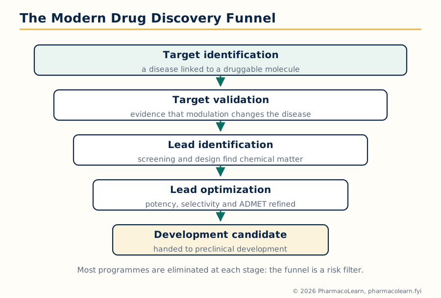 Figure: The modern drug discovery funnel. Programmes narrow stage by stage, and each stage exists to buy the information the next stage spends.
1.2 Target identification: what a drug target is
A drug target is a molecular structure, almost always a protein, whose activity a drug modifies to produce a therapeutic effect. The target classes that dominate marketed medicines are few, and the syllabus's "various targets for drug discovery" objective is met by knowing them:
| Target class | How drugs act | Standard examples of the class at work |
|---|---|---|
| Enzymes | Usually inhibition, often of a disease driving step | HMG CoA reductase (statins), HIV protease (protease inhibitors), angiotensin converting enzyme (ACE inhibitors) |
| G protein coupled receptors | Agonism or antagonism of a signalling receptor | Beta adrenoceptors, histamine H2 receptors, dopamine D2 receptors |
| Ion channels | Block or modulation of ion flow | Voltage gated sodium channels (local anaesthetics), calcium channels (amlodipine) |
| Nuclear receptors | Ligand activated transcription factors | Steroid and thyroid hormone receptors, PPAR gamma (glitazones) |
| Transporters | Block of uptake or transport | Serotonin transporter (SSRIs), proton pump (an enzyme transporter, blocked by PPIs) |
| Structural and other proteins, nucleic acids | Binding that disables a function | Tubulin (vinca alkaloids, taxanes), bacterial ribosome (many antibiotics), DNA itself (alkylating agents) |
A good target needs more than disease association. The working criteria taught with this unit are: efficacy logic (modulating it should change the disease, not merely accompany it); druggability (the protein must possess a site a small molecule can bind with useful affinity; enzymes and GPCRs score well because evolution built them to bind small molecules, while flat protein protein interaction surfaces score badly); assayability (its activity must be measurable in a robust laboratory test, or no screen can be run); selectivity room (it should differ enough from related proteins that a drug can hit it without hitting its cousins everywhere in the body); and a safety margin in principle (a target essential in every tissue is a toxicity risk from the first day). Target identification assembles candidates from disease biology: human genetics, pathway analysis, expression studies in diseased tissue, and the genomics and proteomics methods of sections 1.5 and 1.6.
1.3 Target validation: proving the target deserves a programme
Identification proposes; validation disposes. Target validation is the accumulation of evidence that modulating the target, in the right direction, by a drug like intervention, will produce the desired clinical effect. It is deliberately distinguished from identification because the commonest expensive failure in discovery is a beautifully screened programme against a target that never mattered in patients.
Validation evidence forms a ladder, weakest at the bottom:
- Association: the target is overexpressed, mutated or otherwise abnormal in the disease. Suggestive, never sufficient: the abnormality may be a consequence of the disease rather than a cause.
- Genetic evidence in humans: people carrying loss or gain of function variants in the target gene show the disease, or are protected from it. This is among the strongest early evidence, because nature has already run the experiment of modulating that target for a lifetime.
- Pharmacological evidence: a tool compound, an antibody or a nucleic acid that modulates the target changes the disease process in cells and in animal models, in a dose related and reversible way.
- Genetic manipulation in model systems: switching the target off (knockout, antisense, siRNA) or on, in cells and in transgenic animals (sections 1.9 to 1.11), reproduces or reverses the disease phenotype.
- Clinical proof, the only complete validation: a drug against the target works in patients. It arrives too late to guide the original decision, which is why the earlier rungs must be made as strong as possible.
Two judgements inside validation deserve emphasis. First, direction: the evidence must say whether the target should be activated or inhibited, and programmes have failed by pushing the wrong way. Second, the therapeutic window in principle: a target whose modulation is lethal or intolerable in normal physiology fails validation however elegant the disease logic. Validation is therefore as much a safety discipline as an efficacy one, and it continues during lead optimization, because every toxic lead is also a question about the target.
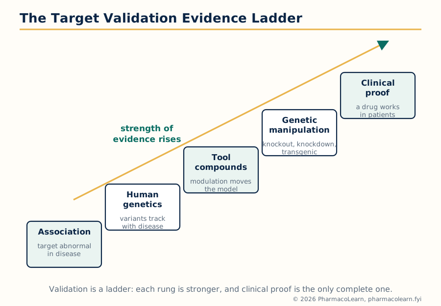 Figure: The target validation evidence ladder. Each rung is stronger than the one below, and only clinical proof completes the validation.
1.4 The economics of drug discovery
The syllabus names the economics of drug discovery as a topic in its own right, and the honest treatment is structural rather than numerical, because published cost estimates differ widely with method and era. The structural facts are stable. Bringing one new medicine to market takes well over a decade from target selection. The overwhelming majority of programmes started are terminated, and the most expensive failures are the late ones, above all in clinical development, where a single large trial costs more than years of discovery work. Discovery itself is therefore run as risk management: money is spent in small, information buying steps early (validation, screening) precisely so that the large sums later are spent on candidates already stripped of every discoverable defect.
Three economic consequences shape the science in this subject. First, fail early and cheap: killing a weak target at validation costs a fraction of killing a weak candidate in Phase II, which is why validation rigour is an economic virtue, not academic caution. Second, the funnel must be wide at the top: because attrition is so high, lead identification screens very large compound collections (Unit 2), and anything that raises the quality of what enters the funnel pays for itself many times over. Third, patent life runs from filing, so years in discovery are years subtracted from protected sales, one pressure behind the computational methods of Units 3 to 5 that promise to shorten the search.
1.5 Genomics in target discovery and validation
Genomics studies the genome as a whole: its sequence, its variation between people, and which genes are switched on or off in a given tissue or disease. Its contributions to target discovery are threefold. First, disease gene discovery: comparing the genomes of patients and controls, through family linkage studies and genome wide association studies, points to genes whose variants track with disease, and each such gene is a candidate target or a signpost to one. Second, target triage: sequence comparison reveals whether a candidate target belongs to a druggable family, whether close relatives exist that threaten selectivity, and whether the same gene is essential in normal tissues. Third, expression genomics: measuring which genes are transcribed in diseased versus healthy tissue (the measurement technology is the nucleic acid microarray of section 1.7) highlights the pathways the disease has disturbed.
Genomics also supplies validation of the strongest kind. A human population carrying a natural loss of function variant in a target gene is a lifelong, whole body experiment in inhibiting that target: if such people are healthy and protected from the disease, the target is validated for both efficacy direction and basic safety in a way no animal model can match. The discipline's limit is equally clear: genes are not proteins, association is not mechanism, and a genomic signal begins, rather than completes, the validation argument.
1.6 Proteomics and bioinformatics
Proteomics applies the same whole system ambition to proteins: identifying and quantifying the full protein content of a cell or tissue, mapping their interactions, and detecting their modifications, typically by separating complex mixtures and identifying the components by mass spectrometry. Where genomics lists what could be made, proteomics reports what is actually present, in what amount, in what modified state, and in whose company, which is closer to the drug target itself, since nearly all targets are proteins. In discovery it serves target identification (proteins abnormally expressed or modified in disease), biomarker discovery (proteins that report disease state or drug response, used to stratify experiments and trials), and mechanism studies (which proteins a candidate drug actually touches, the basis of selectivity screening).
Bioinformatics is the computational discipline that makes both omics usable: storage, alignment and comparison of sequences, prediction of protein families and domains, mining of expression databases, and modelling of pathways. It answers the first questions asked of any candidate target: What family is it? What does its sequence predict about structure and function? Where is it expressed? What happens to organisms that lack it? A target that survives this in silico interrogation earns the expensive wet laboratory work of validation; one that fails it is discarded at the cost of computer time, the cheapest elimination in the whole funnel.
1.7 Nucleic acid microarrays
A nucleic acid microarray (DNA chip) measures the expression of thousands of genes in one experiment. Short DNA probes, each specific to one gene's messenger RNA, are fixed at known positions in a grid on a solid surface. Messenger RNA from the sample is labelled, usually with fluorescence, and allowed to hybridize to the probes; the brightness at each spot reports how much of that gene's message the sample contained. Comparing a diseased sample with a healthy one, spot by spot, yields an expression signature: the pattern of genes turned up or down by the disease.
In target discovery the signature is mined for genes whose change is large, consistent and pathway coherent; such genes, or the proteins they encode, become candidate targets. In validation, the same technology tests whether modulating a candidate target moves the disease signature back toward health. Microarrays also serve pharmacology directly: the expression response of cells to a drug reveals its pathway effects and foreshadows toxicities. Their limitations are those of any messenger RNA measurement: message levels only approximate protein levels, and correlation with disease still has to be converted into causal evidence by the validation ladder of section 1.3.
1.8 Protein microarrays
A protein microarray fixes proteins, rather than nucleic acids, at known grid positions, and asks questions that only proteins can answer. In its common discovery forms, a labelled probe (a candidate drug, an antibody, another protein) is washed over the array, and the spots it binds identify its protein partners. Three uses matter for this subject. First, interaction mapping: which proteins bind a given protein helps place a candidate target in its pathway. Second, drug selectivity profiling: running a lead compound over an array of many proteins exposes off target binding early, when chemistry can still fix it. Third, antibody and biomarker work: arrays of antigens read out the antibody content of patient samples, reporting disease associated immune signatures.
Protein arrays are technically harder than DNA arrays, because proteins denature and lose activity when fixed to surfaces, so each array compromises between coverage and function. They are the protein level counterpart of the nucleic acid array: together the two technologies move discovery from one gene at a time to systems at a time.
1.9 Antisense technologies: antisense oligonucleotides and siRNA
Antisense technologies attack a target at its message rather than at the protein. An antisense oligonucleotide is a short, synthetic, single stranded nucleic acid whose sequence is complementary to the target's messenger RNA. Bound to that message, it blocks protein production, either by recruiting the enzyme RNase H to cut the RNA strand of the hybrid, or by physically blocking splicing or translation. Small interfering RNA (siRNA) reaches the same end by a cellular pathway: a short double stranded RNA is loaded into the RISC complex, one strand is discarded, and the retained strand guides RISC to cut messenger RNAs of matching sequence. In both cases the result is knockdown: a specific, dose adjustable, reversible reduction of one chosen protein, achievable within days of knowing the gene sequence, long before any small molecule inhibitor could exist.
That speed is why the syllabus places these tools inside target validation. If knocking down the target in cells or animals reverses the disease phenotype, validation strengthens; if nothing happens, the target is questioned before a screening campaign is funded. The same mechanisms are also medicines in a small number of diseases where the target tissue can be reached, but their primary discovery role, and the one examined here, is as validation instruments. Their limitations define their use: delivery into cells is imperfect, effects are temporary, and partial knockdown is not identical to full pharmacological blockade of the active site.
1.10 Zinc finger proteins
A zinc finger is a small protein domain, a motif in the language of Unit 2, in which a zinc ion held by cysteine and histidine residues stabilizes a fold that fits into the major groove of DNA. Natural transcription factors string several such fingers together, each finger reading a few base pairs, so that the assembly recognizes one chosen DNA sequence. Because the fingers are modular, they can be engineered: zinc finger proteins built to order can be aimed at a chosen gene and fitted with effector domains that switch the gene off or on, and zinc finger nucleases carry a cutting domain that breaks DNA at the chosen site, allowing a gene to be disrupted or edited in cells and animals.
For drug discovery the value is again instrumental. A zinc finger repressor aimed at a candidate target gene is a validation tool of great precision: it suppresses exactly one gene's expression without chemistry against the protein, complementing antisense and siRNA with a DNA level intervention. Zinc finger nucleases historically provided one route to the knockout animals of the next section. The syllabus includes them as part of the molecular toolkit that modern target validation assumes: genomics finds the gene, and zinc finger reagents let the investigator turn that gene down, off or out, on demand.
1.11 Transgenic animals in target validation
A transgenic animal carries an engineered change in its genome, and in validation work the engineering serves one purpose: to model, in a whole organism, the effect of modulating the target. The standard designs are:
| Design | What is changed | Validation question it answers |
|---|---|---|
| Knockout | The target gene is disrupted so no functional protein is made | What happens when the target is fully inhibited, for life? Mimics a perfect antagonist, and exposes both efficacy logic and on target toxicity |
| Knockin | A modified version of the gene replaces the normal one (a disease mutation, or a drug resistant form) | Does the disease mutation itself cause the phenotype? Does the drug stop working when its binding site is altered, proving on target action? |
| Conditional or inducible knockout | The gene can be switched off in one tissue or at one chosen time | Separates the target's adult pharmacology from its developmental roles, and localises the effect to the tissue that matters |
| Humanized transgenic | The animal gene is replaced by the human version | Tests drugs and biologics that recognise only the human protein |
The interpretive discipline matters as much as the technology. A knockout that produces no disease protection weakens the target, but developmental compensation can hide a real role, since the animal has had a lifetime to rewire around the missing protein; acute blockade or an inducible knockout may reveal what the germline knockout concealed. Conversely, a knockout may exaggerate a drug's effect, because a drug rarely abolishes a protein completely in every tissue. Transgenic evidence sits high on the validation ladder, below human genetics and clinical proof: strong, but not final.
Unit 2: Lead Identification and Protein Structure
2.1 Lead identification: the search for chemical starting points
Lead identification (lead seeking) is the stage that converts a validated, assayable target into chemical matter: compounds with confirmed activity on the target, understood structure, and room to be improved. Its raw materials are compound collections: the accumulated synthetic output of the industry, natural product collections, and libraries built deliberately for screening. Its engines, the three the syllabus names, are combinatorial chemistry, which manufactures candidates at scale; high throughput screening, which tests them at scale; and in silico lead discovery, which searches them, and virtual libraries far larger, by computation before any bench work. All three feed on one prerequisite: a trustworthy assay, which is where this unit begins in practice.
2.2 Assay development for hit identification
An assay is the laboratory measurement that reports whether a compound acts on the target. Everything downstream is only as good as this measurement, so assay development is a discipline in itself. The assay must reproduce the relevant biology in miniature: for an enzyme target, the purified protein converting substrate to product; for a receptor, binding of a labelled ligand or a cellular signal downstream of activation; for a cell based question, a phenotype such as growth, death or reporter gene expression in the disease relevant cell.
| Assay design choice | Options | Consequences |
|---|---|---|
| Biological level | Biochemical (isolated target) vs cell based (target in its cellular context) | Biochemical assays are clean, cheap and fast but blind to membrane permeability and cell toxicity; cell based assays are realistic but noisier and slower, and a hit may act anywhere in the pathway |
| Readout | Radioactivity, fluorescence, luminescence, absorbance, label free methods | Must be robust at screening scale, cheap per well, and free of interference by the test compounds themselves (coloured or fluorescent compounds are a classic false positive source) |
| Format | Plate based, miniaturized (384 or 1536 wells), automated liquid handling | Miniaturization cuts cost per test by orders of magnitude and makes million compound screens feasible |
| Quality control | Positive and negative controls on every plate, signal window, the Z prime statistic comparing control separation with control variability | A Z prime value comfortably above 0.5 marks an assay fit for screening; below that, hit lists are mostly noise |
A developed assay is hardened by counter screens: parallel tests that discard compounds acting by nuisance mechanisms, such as inhibiting the reporter rather than the target. A hit survives this gauntlet: reproducible, concentration dependent activity, confirmed on retest from fresh material, of known structure. The hit rate of a well run screen is a small fraction of one percent of the library, and hits pass to the further filters of section 2.6.
2.3 Combinatorial chemistry
Combinatorial chemistry is the systematic synthesis of large sets of related compounds (libraries) by combining sets of building blocks in every, or nearly every, possible combination. If ten variants of one component react with ten of a second and ten of a third, the arithmetic gives a thousand products from thirty building blocks: chemistry by multiplication. Two execution styles dominate:
- Parallel synthesis: each compound is made separately, in its own well or vessel, as a single pure product of known identity. Libraries are smaller but every member is identified and immediately testable.
- Split and mix (split and pool) synthesis: resin beads are divided into portions, each portion reacts with one building block, the portions are pooled and mixed, and the cycle repeats. Each bead ends carrying one compound, built by its own route through the pools; the library is enormous (hundreds of thousands to millions) but the identity of the compound on a given bead must be decoded or the active mixture deconvoluted by resynthesizing sub libraries.
Combinatorial chemistry transformed lead identification by guaranteeing that a screen always had matter to test, and it pairs naturally with high throughput screening: one manufactures the library, the other interrogates it. Its historical lesson also belongs in the notes: size alone did not raise success, because libraries built for easy synthesis clustered in flat, greasy, similar chemistry that made poor leads. Modern libraries are designed for diversity and for drug like properties, applying the filters of Unit 3 at the drawing board.
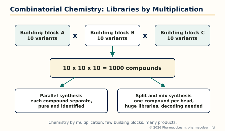 Figure: Combinatorial chemistry multiplies a few building blocks into a library of thousands, made by parallel synthesis or by split and mix.
2.4 High throughput screening
High throughput screening (HTS) is the automated testing of very large compound collections against the assay of section 2.2. Robotic liquid handlers dispense nanolitre volumes into miniaturized plates, incubators and plate readers process them in sequence, and software assembles the results into ranked activity lists. At full industrial scale a screen can test on the order of a hundred thousand compounds in a day, and a full collection in weeks, a rate unthinkable for the manual pharmacology of earlier units.
A HIGH THROUGHPUT SCREEN, WELL BY WELL

  Compound library (plates of single compounds in DMSO)
      |
      v
  Robotic dispensing into assay plates -- target + reagents added
      |
      v
  Incubation, then plate reader measures the signal
      |
      v
  Software: % inhibition per well, plate quality controls checked
      |
      v
  Primary hits -> retest in duplicate -> dose response curves
      |
      v
  Counter screens remove nuisance actives
      |
      v
  Confirmed hits -> hit to lead chemistry
HTS is powerful and credulous in equal measure, and the syllabus's pairing of it with assay development is the point. It reports whatever the assay measures, including artefacts: compounds that fluoresce like the product, quench the signal, aggregate into colloidal particles that sequester the protein nonspecifically (a notorious source of promiscuous false hits), or react covalently with assay components. Hit triage, with fresh powder retests, dose response curves, detergent controls and orthogonal assays measuring the same biology by a different readout, is therefore part of HTS rather than an afterthought. HTS also returns in Unit 3, inside rational design.
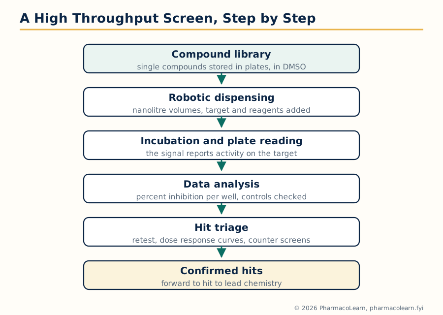 Figure: A high throughput screen, step by step, from stored library plates to confirmed hits after triage.
2.5 In silico lead discovery techniques
In silico lead discovery searches for leads by computation before, or instead of, bench screening. Its main techniques, developed fully in Units 3 and 4, are introduced here as lead seeking methods: similarity searching, which finds library compounds resembling a known active; pharmacophore screening, which searches for molecules presenting the same arrangement of chemical features as known actives; molecular docking, which predicts how each library member would sit in the target's binding site and ranks them by computed fit; and property filtering, which removes compounds whose predicted solubility, permeability or toxicity make them hopeless as leads whatever their activity.
The strategic value is leverage. A physical collection numbers in the millions; a virtual collection, enumerated on a computer, can be far larger, and in silico screening costs computer time rather than robotics and reagents. Its discipline is that every prediction is a hypothesis: in silico hits must still be bought or made and tested in the real assay, and the method earns its place by enriching that test set, delivering a far higher hit rate among the compounds actually assayed than random selection would.
2.6 From hits to leads: what a lead must be
Not every confirmed hit deserves a chemistry programme. The hit to lead step applies the criteria that separate a lead series from a screening curiosity:
- Confirmed, tractable potency: activity strong enough to improve (typically at least micromolar, with a clean dose response), in a series where analogues can be synthesized to explore structure activity relationships.
- Selectivity at birth: meaningful preference for the target over its closest relatives and over standard nuisance panels, or at least a structural reason to believe selectivity can be built.
- No structural alerts: freedom from reactive, unstable or promiscuously binding chemotypes that will poison optimization later.
- Drug like physicochemistry: solubility and lipophilicity in ranges compatible with the drug likeness rules of Unit 3; potency bought with excessive lipophilicity is a debt, repaid later as poor solubility and promiscuity.
- Novelty and freedom to operate: a series already patented by a competitor is scientifically interesting and commercially useless.
A series meeting these tests is declared a lead, and lead optimization (section 1.1) begins. The rest of this unit supplies the structural knowledge that both hit assessment and optimization increasingly rely on: the three dimensional structure of the target protein.
2.7 Protein structure: why discovery runs on it
Nearly every method in Units 3 and 4 consumes protein structure. Docking needs the coordinates of the binding site; pharmacophore models of a target need to know which residues offer hydrogen bonds; lead optimization explains each potency change by what the structure shows. When the structure of the target itself is unavailable, the structure of a relative may serve, and when none exists, computational prediction (sections 2.11 and 2.12) attempts to supply one. This half of Unit 2 therefore covers what protein structure is, how it is described, and how it is determined or predicted.
2.8 Levels of protein structure
Protein architecture is described at four levels:
| Level | Meaning | What holds it together |
|---|---|---|
| Primary structure | The amino acid sequence, read from the N terminus to the C terminus | Peptide bonds; sequence alone, determined by gene sequencing and mass spectrometry |
| Secondary structure | Local regular folding of the chain: alpha helices, beta strands and sheets, turns and loops | Hydrogen bonds between backbone carbonyl and amide groups |
| Tertiary structure | The complete three dimensional fold of one polypeptide chain | Hydrophobic packing of side chains into a core, hydrogen bonds, ionic interactions, van der Waals contacts, and disulfide bonds between cysteines |
| Quaternary structure | The assembly of several folded chains (subunits) into one functional complex | The same non covalent forces as tertiary structure, acting between subunits, as in haemoglobin's four chains |
The drug binding site is a tertiary (sometimes quaternary) feature: a pocket or groove whose shape and chemistry are created by residues far apart in sequence but adjacent in the fold. That single fact explains both why sequence alone rarely predicts druggability and why the experimental structures of sections 2.13 and 2.14 are so prized.
2.9 Domains, motifs and folds
Between the whole chain and the single residue sit three descriptive units the syllabus names. A domain is a segment of the chain that folds independently into a compact structure and usually carries one function: the kinase domain that phosphorylates, the SH2 domain that reads phosphotyrosine marks. Domains are the reusable bricks of protein evolution, and druggable pockets very often sit in or between domains. A motif (sequence motif) is a short conserved pattern of amino acids that signals a function: the zinc finger of section 1.10 is a motif, as is the Walker motif of ATP binding proteins; motifs are recognized from sequence and are the working vocabulary of bioinformatics. A fold is the overall three dimensional arrangement of secondary structures in a domain (for example the Rossmann fold of many nucleotide binding domains), and unrelated sequences can converge on the same fold while related sequences nearly always share one. The distinction matters practically: fold is conserved longer than sequence, which is the opening that threading (section 2.12) exploits.
2.10 Computational prediction of protein structure: the problem
Experimental structure determination is slow and sometimes impossible (membrane proteins, the largest target class, resist both crystallography and NMR). Computational prediction attempts to build a usable model from sequence alone. The methods divide by how much help the sequence receives from known structures. If a related protein of known structure exists, homology modelling copies and adapts it. If no relative is detectable by sequence, threading tests whether the sequence could adopt any known fold. Both are syllabus methods; both produce models, not structures, and a model's value depends on how it is validated and what question it is asked to answer. A model good enough to suggest which residues line a pocket, and to design the experiment that tests the suggestion, has earned its keep even if its details are approximate.
2.11 Homology modelling
Homology modelling (comparative modelling) builds a model of a target protein from the experimental structure of a homologous protein, the template, on the principle that structure is conserved more strongly than sequence: two proteins of clearly similar sequence fold the same way. The standard steps are:
HOMOLOGY MODELLING, STEP BY STEP

  1. Template search: find proteins of known structure related
     to the target sequence (sequence database searching)
      |
  2. Sequence alignment: line the target sequence up with the
     template so equivalent residues correspond
      |
  3. Model building: copy the template backbone for aligned
     regions; build the differing loops; place side chains
      |
  4. Refinement: energy minimization settles clashes and strains
      |
  5. Validation: geometry checks, eg the Ramachandran plot,
     should show a protein like model; implausible regions
     are realigned and rebuilt
Accuracy tracks relatedness. With a close template (high sequence identity over the whole chain) the backbone of the model approaches experimental usefulness and docking into it is routine; with a distant one, only the conserved core is trustworthy and the loops, often including the binding site rim, carry large errors. The alignment is the step where most error enters: a single shifted residue in the alignment misplaces every atom built on it, which is why experienced modellers spend their effort there and validate before they dock.
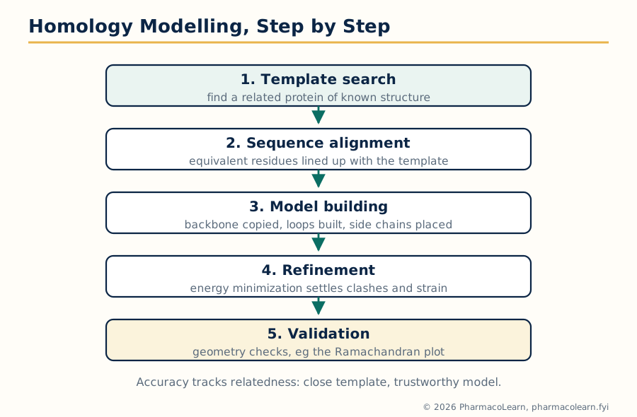 Figure: Homology modelling in five steps. The sequence alignment is the foundation: errors made there cannot be repaired by later refinement.
2.12 Threading and fold recognition
Threading answers the question homology modelling cannot: when no sequence relative with known structure can be found, does the target sequence fit any known fold at all? The target sequence is threaded, in imagination, through each fold in a library of known structures, and each trial fit is scored by how happily the sequence sits in that environment: hydrophobic residues buried, polar residues exposed, favourable residue pair contacts. The best scoring fold is adopted as the predicted architecture, and a model is built on it.
Threading trades resolution for reach. It can identify the correct fold family for a protein with no detectable sequence relatives, because structure tolerates sequence change better than alignment statistics tolerate it, but it cannot deliver atom level confidence: side chain placement and loop detail remain speculative. Its discovery use is therefore triage and hypothesis generation, for example predicting that a new target is a kinase fold protein and should be screened and modelled as one, rather than supplying coordinates for precision docking.
2.13 NMR spectroscopy in protein structure determination
Nuclear magnetic resonance determines protein structures in solution, the state closest to physiology. In outline: the protein is labelled with the NMR active isotopes nitrogen 15 and carbon 13, a battery of multidimensional experiments assigns each resonance to a specific atom, and experiments that detect through space proximity (the nuclear Overhauser effect) yield thousands of approximate distances between atom pairs. Computational folding then finds the family of structures consistent with those distances, angles and couplings, and the structure is reported as an ensemble of conformers rather than one rigid pose, honestly reflecting molecular motion.
NMR needs no crystals, works in solution, and reports dynamics and weak interactions, which is why it also serves ligand screening directly: methods that watch ligand signals report binding and can locate it on the protein. Its limits are size and labour: proteins much above roughly 30 to 40 kilodaltons broaden into unreadability, and throughput is low. In discovery, NMR structures are most prized for small domains and for the dynamic questions rigid crystal structures cannot answer.
2.14 X-ray crystallography in protein structure determination
X-ray crystallography remains the source of most protein structures in the public databases and the workhorse of structure based design. The protein is persuaded to form an ordered crystal, a regular lattice of many copies; X-rays scattered by the crystal produce a diffraction pattern; and computation converts that pattern into an electron density map into which the atomic model is built and refined. The map's sharpness is quoted as resolution: at resolutions around 2 angstroms or better, individual atoms and ordered water molecules are placed with confidence sufficient for drug design.
Three features make crystallography a discovery engine rather than merely a measurement. First, soaking and co crystallization: crystals of the target with a lead bound show exactly how the drug sits and which interactions it makes or misses, turning each potency puzzle of lead optimization into a structural instruction. Second, throughput: once a crystallization system exists, structures of dozens of analogues can follow in the design cycle. Third, the Protein Data Bank archive supplies the templates for homology modelling and the folds for threading, so crystallography underpins even the computational methods. Its limits are the crystal itself: some proteins refuse to crystallize, flexible regions vanish from the map, and the lattice can hold a conformation the cell never uses, which is why crystallographic claims are cross checked against solution methods where the answer matters.
Unit 3: Rational Drug Design and Virtual Screening
3.1 Traditional drug design: discovery before targets
For most of pharmaceutical history there was no target to design against. Traditional drug design found drugs by their effects in whole organisms, tissues or, later, crude biochemical tests, and understood their mechanisms afterwards, if at all. Its sources were the materia medica of traditional medicine, the dye and chemical industries, and chance. Its logic was phenotypic: a substance that relieved the observable disease sign was a lead, whatever it touched.
The method was far from barren. Morphine was isolated from opium, quinine from cinchona bark, and testing natural materials in patients and animals delivered much of the older pharmacopoeia. Penicillin arrived by famous serendipity, a contaminated plate noticed by an observant scientist, and the sulfonamides emerged from screening industrial dyes, the screening that revealed Prontosil. Traditional design's systematic weakness was the mirror of its strength: with no mechanism, optimization was blind chemistry around a scaffold, toxicity and inefficacy were discovered late, and whole classes of mechanism that whole animal tests cannot see were unreachable.
3.2 Methods followed in traditional drug design
The PCI syllabus asks for the methods of the traditional approach explicitly, and they form a coherent toolkit:
- Random or phenotypic screening: collections of natural products, plant extracts and synthetic compounds are tested in disease relevant whole animal or tissue models, and activity, not mechanism, selects the hits.
- Serendipity and clinical observation: unexpected effects noticed in the clinic are converted into new indications. The standard history is sildenafil, developed as a candidate for angina, whose observed side effect in trials redirected it to erectile dysfunction, a change of indication no screen would have requested.
- Analogue synthesis around an existing drug (me too and me better design): modifying a proven drug's structure to improve potency, duration, safety or patent position, learning from the predecessor's weaknesses. Much of the sulfonylurea, benzodiazepine and statin families grew this way.
- Exploiting side effects and metabolites: a drug's secondary action or its active metabolite becomes the starting point of a new programme, separating the wanted effect from the parent molecule.
- Folk and ethnobotanical leads: traditional remedies are tested and their active principles isolated and purified, the path of morphine, digoxin and, in the modern era, artemisinin.
Each method shares one property: the molecule is found before its target is known, and the target, sometimes, is only identified decades later. That inversion of the modern order is the cleanest definition of the traditional approach.
3.3 Rational drug design: the concept
Rational drug design inverts the traditional order. It begins from knowledge: of the disease mechanism, of the target's identity and ideally its structure, and of the chemistry of the interaction to be created or blocked. The drug is then designed, on paper and on screen, to fit that knowledge, synthesized, and tested against predictions. Two classical programmes mark the transition and are the standard teaching examples. Captopril was designed from a snake venom peptide that inhibited angiotensin converting enzyme and from the known active site chemistry of a related enzyme, carboxypeptidase A: a small molecule was drawn to present the same binding features, and it worked as drawn. Cimetidine was built by systematically modifying histamine itself, step by rational step, until agonism at the newly distinguished H2 receptor had been converted into antagonism. In both, hypothesis preceded synthesis, which is the essence of the rational claim.
Rational design does not abolish empiricism; it relocates it. Screening still tests designs, and most designs still fail, but each failure now tests a stated hypothesis and returns usable information. The comparison the syllabus demands is summarized below.
| Feature | Traditional drug design | Rational drug design |
|---|---|---|
| Starting point | Observed effect in organism or tissue | Knowledge of target and disease mechanism |
| Target known at start | Usually no; identified later or never | Yes; identification and validation precede chemistry |
| Role of screening | The discovery engine itself | A tool for testing designed or selected candidates |
| Optimization guided by | Activity and tolerability in whole systems | Structure, mechanism and quantitative relationships |
| Strength | Finds the unexpected; no assumptions about mechanism | Focused, information rich, reaches mechanisms invisible to whole animal tests |
| Weakness | Blind, slow, late toxicity, mechanism free | Fails completely if the target hypothesis is wrong; needs structures and assays traditional work did not |
3.4 High throughput screening within rational design
HTS appears in this unit as well as Unit 2, and the double appearance is instructive. In the rational era, HTS is no longer random fishing: the target has been chosen and validated rationally, the assay designed against it deliberately, the library curated for drug likeness. The screen is empirical in execution and rational in architecture, and this hybrid is how most modern programmes begin. The examination distinction to retain is that HTS is a technique, usable by either philosophy, while rational design is a philosophy about the order of knowledge and experiment.
3.5 Structure based drug design
Structure based drug design (SBDD) is the rational method that designs from the three dimensional structure of the target, obtained by X-ray crystallography or NMR (Unit 2) or by a validated model. Knowing the binding site's shape, its hydrogen bond donors and acceptors, its hydrophobic surfaces and its charged residues, the designer either builds a molecule to complement them (de novo design, Unit 4) or selects and modifies existing molecules by docking them in the site computationally. The working cycle is iterative: structure of target with lead bound, design a change, synthesize, test, new structure. The HIV protease inhibitors are the canonical success of the method: the viral enzyme's structure was solved early, its symmetric active site was unlike any human protease, and inhibitors were designed against the structure to clinical effect. SBDD's precondition is written into its name: without a structure, or a model of homology modelling quality, there is nothing to base the design on, and the programme must fall back on the ligand based methods.
3.6 Pharmacophore based (ligand based) design
When several compounds are known to act on a target but the target's structure is unknown, the common pattern among the actives themselves becomes the design guide. A pharmacophore is that pattern: the spatial arrangement of chemical features, hydrogen bond donors and acceptors, hydrophobic groups, aromatic rings, charged centres, that a molecule must present to bind. Pharmacophore based design builds this model from the active molecules (mapping is treated fully in section 3.8), then uses it to design new molecules that present the same features on different skeletons, and to screen databases for them. Because it needs no protein structure, it was historically the first rational method available for most targets, and it remains the method of choice when the target is a membrane protein whose structure resists experiment. Its weakness is shared with all inference from examples: the model explains the compounds it was built from, and unusual new chemistry may bind in ways the feature pattern never imagined.
3.7 Virtual screening: the concept and the cascade
Virtual screening is the in silico counterpart of HTS: a large collection of compounds, existing only as computed structures, is passed through a sequence of computational filters of increasing cost and sophistication, and the survivors, a few hundred at most, are purchased or synthesized and tested in the real assay. A typical cascade runs:
THE VIRTUAL SCREENING CASCADE

  Virtual library (millions of structures)
      |
      v
  Drug likeness and property filters remove the hopeless
      |
      v
  Pharmacophore search or similarity search selects the plausible
      |
      v
  Docking ranks the survivors by predicted fit to the target
      |
      v
  Human inspection: chemistry sense, diversity, no artefacts
      |
      v
  A few hundred compounds -> real assay -> real hits
Each stage discards most of what reaches it, exactly as a physical screen's funnel does, but at computing prices. The result is judged by enrichment: a virtual screen returning actives at many times the random rate has done its job, even though most selections still fail in the assay. Virtual screening complements rather than replaces HTS: it reaches chemical space no physical collection contains, but its rankings carry model error everywhere, which the assay alone corrects.
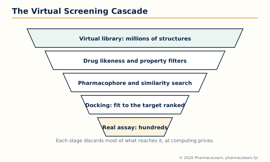 Figure: The virtual screening cascade. Each computational stage discards most of what reaches it, so the expensive real assay is spent on hundreds, not millions.
3.8 Drug likeness screening
The cheapest filter in the cascade is drug likeness screening: the removal, before any target specific test, of compounds whose general properties make them unlikely ever to become acceptable oral drugs. Its famous codification is Lipinski's rule of five, distilled from the properties of marketed oral drugs: poor absorption or permeation becomes more likely when a compound has molecular weight above 500, calculated log P above 5, more than 5 hydrogen bond donors, or more than 10 hydrogen bond acceptors. A related refinement adds limits on rotatable bonds (flexibility) and polar surface area, which govern the same permeability behaviour.
The rules are used as flags, not laws, and the examination nuance matters. They describe a statistical tendency of oral small molecules, not a definition of a drug: many successful medicines violate a rule, especially natural products and drugs for non oral routes or transporter carried drugs, and rigid enforcement would have deleted them. In screening practice a single violation warns, two violations argue strongly against a lead series, and properties are rechecked at every optimization step, because medicinal chemistry has a known tendency to buy potency with size and lipophilicity until the rule of five debt comes due.
3.9 Pharmacophore mapping
Pharmacophore mapping is the disciplined construction of the pharmacophore model of section 3.6. The steps are: assemble a training set of active compounds, ideally spanning a range of potencies and chemotypes; generate, for each, the set of conformations it can realistically adopt; identify the chemical features each molecule offers (hydrogen bond donor, hydrogen bond acceptor, hydrophobic centre, aromatic ring, positively or negatively ionizable group); and then search for an arrangement of features, with distances and angles between them, that some accessible conformation of every active can present simultaneously. Features shared by all actives and absent in inactives are weighted most; the finished model is a three dimensional query: a map of what a binder must look like, drawn in features rather than atoms.
Two refinements complete the practical method. Exclusion volumes mark space that inactive compounds occupy and actives avoid, modelling the walls of the binding site without any protein structure. And the model is validated like a QSAR: it must retrieve known actives from a database seeded with inactives, and fail to retrieve the inactives, before it is trusted to screen.
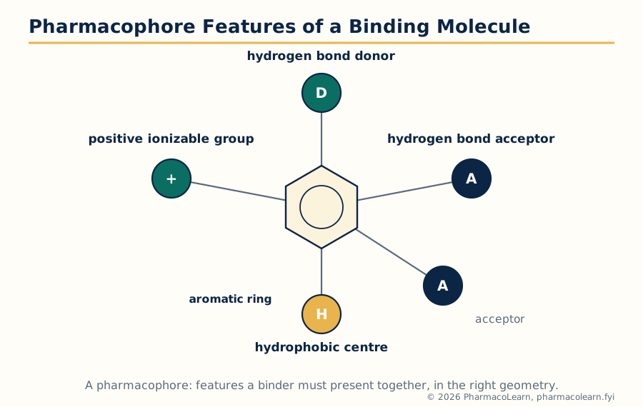 Figure: The features of a pharmacophore: a donor, acceptors, a hydrophobic centre, an ionizable group and an aromatic ring, held in the geometry the target demands.
3.10 Pharmacophore based screening
Pharmacophore based screening runs the validated pharmacophore as a three dimensional search query against databases of computed compound conformations. Every database molecule whose conformers can present the required features, within tolerance, in the required geometry is returned as a candidate hit. The method's distinctive prize is scaffold hopping: because the query is written in features, not atoms, it retrieves molecules whose skeletons differ completely from every training compound while presenting the same binding pattern. A programme trapped in a patented or toxic chemotype can thereby jump to fresh chemistry without losing the binding logic, something neither similarity searching, which stays near known matter, nor analogue synthesis can do. Retrieved hits are then filtered for drug likeness, docked if a structure exists, and tested, entering the ordinary hit to lead gauntlet of section 2.6.
Unit 4: Molecular Docking, De Novo Design and QSAR Foundations
4.1 Molecular docking: what the computation attempts
Molecular docking predicts the bound geometry (the pose) of a small molecule in a target's binding site, and estimates how well it binds (the score). It is the engine inside structure based design and docking based screening. Every docking method solves two coupled problems. Sampling searches the space of possible poses: the ligand can sit in the site in many positions, rotations and conformations, and the protein may adjust around it. Scoring evaluates each sampled pose with a scoring function that estimates binding affinity from the interactions the pose makes. Docking fails in the two corresponding ways: the correct pose was never sampled, or it was sampled but scored below wrong poses. The three syllabus methods are points on the sampling spectrum.
4.2 Rigid docking
In rigid docking, both ligand and protein are treated as rigid bodies: the ligand's precomputed conformation is placed into the site in every orientation, and complementarity of shape and chemistry is scored. It is the fastest possible docking, able to process very large libraries, and historically the first form (the lock and key picture made computational). Its flaw is the premise: real ligands flex and real sites breathe, so a rigid search misses poses the flexible molecule would find and rejects compounds whose bound conformation differs from the one supplied. Rigid docking survives as a first pass filter in large screens, where its speed removes the obviously impossible before flexible methods spend time on the plausible.
4.3 Flexible docking
Flexible docking allows the ligand to change conformation during the search, exploring its rotatable bonds while it is placed, so the pose found is a genuine bound conformation rather than a precomputed guess. The protein is usually held rigid, or granted limited flexibility in the side chains lining the site, because full protein flexibility multiplies the search space beyond routine computation. Allowing the protein to adjust to the ligand is the induced fit problem, and the most capable protocols treat selected side chains as movable or dock against several protein conformations. Flexible docking is the standard working method: slow relative to rigid docking, honest relative to everything the ligand actually does, and accurate enough on redocking tests, where a ligand removed from its crystal structure is usually returned within about 2 angstroms of its true pose, to be trusted for ranking within a programme.
4.4 Manual docking
Manual docking places the ligand in the site interactively, by a scientist using molecular graphics: rotating and adjusting the molecule by eye and chemical judgement, inspecting clashes and unsatisfied hydrogen bonds in real time. It is the oldest form of docking, and it survives because it does what algorithms do badly: incorporate everything the scientist knows, the assay quirks, the analogue data, the suspicion that a residue moves, into one placement decision. Its costs are throughput and reproducibility, so its modern role is hypothesis building and the careful hand examination of the few compounds that matter most.
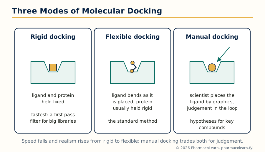 Figure: Rigid, flexible and manual docking compared: realism rises and speed falls from the first to the second, and judgement enters with the third.
4.5 Scoring functions and their limits
A scoring function converts a pose into a number meant to track binding affinity. The families in standard use estimate affinity from force field terms (van der Waals and electrostatic energies of the pose), from empirical terms fitted to measured affinities of known complexes (hydrogen bonds, hydrophobic burial, entropy penalties for frozen rotatable bonds), or from knowledge based potentials distilled from the geometry statistics of many crystal structures. All three share the same honest limitation: they rank far better than they measure. A score can order a series so the best poses rise to the top, which is all screening asks, but it does not deliver a trustworthy absolute affinity, because solvent effects, protein motion and entropy are approximated crudely. Docking therefore concludes with inspection and experiment, never with the score alone, and consensus scoring, requiring several functions to agree, is a common defence against any one function's blind spots.
4.6 Docking based screening
Docking based screening is virtual screening (section 3.7) with docking as its engine: a library is docked into the target's site and ranked, and the top fraction is selected for assay. Performance is measured by enrichment of true actives in that top fraction over random selection, and the method is validated before use by redocking the co crystallized ligand (which must return close to its experimental pose) and by checking that known actives outrank property matched decoys. Used well, it finds chemotypes similarity methods cannot, because it judges fit to the site rather than resemblance to known ligands. Used carelessly, against a poor structure or with artefacts unfiltered, it fills the assay plate with implausible molecules that score well in the computer and nowhere else, which is why drug likeness filtering and human inspection flank it in the cascade.
4.7 De novo drug design
De novo design builds the ligand inside the site from scratch. Fragments or atoms are placed at the site's interaction hot spots, the places where hydrogen bond partners, hydrophobic contacts or charges are offered, and then grown or linked into a complete molecule that satisfies them all, under the discipline of valence and synthetic sense. Where docking selects from what exists, de novo design proposes what should exist, and its proposals routinely include chemotypes no library contains.
Its acknowledged weakness is the last step: a structure elegant in the site may be a nightmare to synthesize, or unstable, or insoluble. Modern practice therefore constrains the builder with synthetic accessibility rules and fragment libraries of purchasable pieces, and treats de novo output as inspired starting points for medicinal chemists rather than finished candidates. As a syllabus method it completes the structure based trio: docking tests the known, pharmacophores abstract the known, de novo design invents the new.
4.8 QSAR: history and development
A quantitative structure activity relationship (QSAR) expresses biological activity as a mathematical function of a molecule's physicochemical or structural properties, so that activity can be predicted for unsynthesized analogues. Its development, as the syllabus requires, runs in clear steps. In the nineteenth century Crum Brown and Fraser proposed that physiological activity is a function of chemical constitution, the founding idea. Around 1900 Meyer and Overton independently found that narcotic potency tracks oil water partitioning, the first quantitative property relationship and the ancestor of the lipophilicity parameter. Hammett, in the 1930s, gave physical organic chemistry its electronic parameter, sigma, and a linear free energy equation for reactivity. The modern subject begins in the early 1960s, when Hansch combined these strands, lipophilicity, electronic and steric terms in one regression equation for biological activity, and Free and Wilson published their additive substituent model in the same era. From those two foundations grew the statistical apparatus of Unit 5 and, in the 1980s, the three dimensional extension CoMFA.
4.9 SAR versus QSAR
The distinction the syllabus draws is between reading a pattern and fitting an equation:
| Feature | SAR (structure activity relationship) | QSAR (quantitative SAR) |
|---|---|---|
| Form | Qualitative: statements about what structural changes raise or lower activity | Quantitative: an equation relating measured activity to numerical parameters |
| Typical statement | A para halogen increases potency in this series | log (1/C) = 0.9 log P - 0.4 sigma + 2.1, with stated statistics |
| Data needed | A handful of analogues and their activities | A congeneric series with reliable activities and computed or measured parameters, enough compounds to support statistics |
| What it gives | Design intuition and hypotheses | Predictions for untested analogues, and an optimum (for example of log P) to design toward |
| Risk | Over reading single pairs of compounds | Over fitting: an equation that describes the data but predicts nothing, controlled by the statistics of Unit 5 |
SAR is the older and universal habit of medicinal chemistry; QSAR is SAR made numerical and therefore testable, at the price of assumptions the next sections state.
4.10 Physicochemical parameters
QSAR equations are built from parameters, numbers that capture one property of a substituent or molecule. The three classical families are:
| Family | Parameter | What it measures |
|---|---|---|
| Hydrophobic | log P (partition coefficient of the whole molecule), and pi, the contribution of one substituent to log P relative to hydrogen | Tendency to leave water for a lipid like environment; governs membrane crossing and hydrophobic binding |
| Electronic | Hammett sigma: sigma para and sigma meta describe a substituent's electron withdrawing (positive) or donating power; related constants describe field and resonance components | The electron density a substituent creates at a reaction or binding centre, influencing ionization and interaction strength |
| Steric | Taft Es (from rates of acid catalysed ester hydrolysis), molar refractivity (MR, size combined with polarizability), and simple size descriptors | The space a substituent occupies and the crowding it causes near the binding interaction |
Parameters come from experiment on model systems or from computation, and the parameter tables compiled for common substituents are what make Hansch analysis practical: a new analogue's pi, sigma and Es are looked up or computed, never measured from scratch.
4.11 Hansch analysis
Hansch analysis fits, for a congeneric series acting by one mechanism, an equation of the form:
log (1/C) = a (log P) - b (log P)^2 + c (sigma) + d (Es) + constant
where C is the molar concentration producing the defined effect, so that log (1/C) rises with potency. Each term carries a physical story. The log P terms are characteristically parabolic: potency first rises with lipophilicity, as the molecule partitions more readily toward its site, then falls as it becomes too greasy to dissolve, travel and leave depot phases, so the equation contains an optimum log P for the series, one of the most useful single numbers classical QSAR produces. The sigma term reports whether electron donation or withdrawal at a position helps binding; the Es term penalizes or rewards bulk near the pharmacophore. The coefficients are found by regression (Unit 5) and are believed only when the statistics, the number of compounds per parameter, and the mechanism constancy of the series support them. The method's lasting legacy is conceptual as much as numerical: it taught medicinal chemistry to think of potency as a balance of transport and binding properties that can be optimized separately and deliberately.
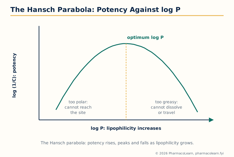 Figure: The Hansch parabola. Potency peaks at an optimum log P and falls on both sides, too polar on the left and too greasy on the right.
4.12 Free Wilson analysis
Free Wilson analysis takes the opposite route to the same quantity. It assumes a series built on a common scaffold with substituents varied at defined positions, and it models activity as the sum of a contribution from each substituent at each position plus the activity of the unsubstituted parent:
log (1/C) of an analogue = parent (mu) + sum of substituent contributions
A teaching miniature fixes the arithmetic exactly. Suppose the parent compound has log (1/C) = 4.00, a para chloro substituent contributes +0.42 wherever the analysis has established it, and a meta methyl contributes -0.18. The analogue carrying both is predicted at 4.00 + 0.42 - 0.18 = 4.24, without any measurement. The contributions are extracted from the series itself by regression on indicator variables (present or absent), so the method needs no physicochemical tables and no property assumptions. Its demands are combinatorial instead: the series must vary substituents at each position sufficiently independently for their contributions to be separable, and the model is mute about any substituent never made. Additivity is its wager: where substituents interact, for example one changing the ionization another depends on, the sum errs, and the method says so through its residuals.
4.13 The relationship between Hansch and Free Wilson analysis
The two methods are relatives, and the syllabus asks for the relationship explicitly. Formally, a Free Wilson indicator variable for a substituent behaves like a Hansch parameter that is switched on by that substituent's presence; when a substituent's Hansch parameters (its pi, sigma, Es) are themselves used to explain its Free Wilson contribution across many series, the two descriptions meet. Fujita's mixed approach operationalizes the union: an equation containing physicochemical parameters for the positions where property logic is trusted, and indicator variables for the positions where it is not. Practically, the choice is pragmatic. Hansch analysis generalizes: from the equation, the activity of a substituent never synthesized can be estimated from its parameter values. Free Wilson analysis is self contained and assumption light, but it can only recombine substituents already present in the data. Modern QSAR descends from both: the descriptors changed, the statistics deepened (Unit 5), and the additivity and property balance ideas remained.
Unit 5: QSAR Statistics, 3D QSAR and Prodrug Design
5.1 The statistical contract of QSAR
A QSAR equation is a statistical claim before it is a chemical one, and Unit 5 supplies the machinery for judging it. The contract has three clauses. First, enough data: a working rule is at least five compounds per fitted parameter, since each added term will improve the fit to the data in hand whether or not it captures anything real. Second, honest significance: the statistics of section 5.2 must show the fit exceeds what chance correlation among random numbers would produce. Third, demonstrated prediction: the equation must predict compounds it was not fitted on, tested by the validation discipline of section 5.5. An equation meeting all three is a model; one meeting only the first two is a description.
5.2 Regression analysis
Regression analysis, in QSAR almost always multiple linear regression, finds the coefficients of the Hansch type equation that minimize the squared differences between observed and calculated activities. The output is judged by a standard battery:
| Statistic | Meaning | Healthy sign |
|---|---|---|
| r, the correlation coefficient (and r squared) | Fraction of the variation in activity the equation accounts for | r squared above about 0.8 for a working model, read with the other statistics, never alone |
| s, the standard deviation of the residuals | Typical size of the equation's error, in activity units | Comparable to the experimental error of the biological measurements themselves; it cannot honestly be much smaller |
| F, the variance ratio | Whether the explained variance dwarfs the unexplained, given the numbers of compounds and parameters | Large, and significant at a strict level; punishes equations that buy fit with parameters |
| Residual pattern | The signs and sizes of individual errors across the series | No structure: a curved residual pattern is the equation confessing a missing term, as when a linear log P fit leaves a parabola in its errors |
Regression also carries the standard warnings of the method: it assumes the parameters are measured without major error and independent enough to be separable, and with many candidate parameters and few compounds it will find a flattering equation by chance, the chance correlation problem that the five to one rule and cross validation exist to restrain.
5.3 Partial least squares analysis
Partial least squares (PLS) is the multivariate method that succeeds regression where regression fails: when the descriptors are numerous and highly correlated with one another. Instead of using the raw descriptors, PLS constructs a small number of latent variables, weighted combinations of many descriptors, each chosen to capture the maximum remaining covariance with activity, and the model regresses activity on a handful of these components. Two consequences follow. The method tolerates descriptor counts far exceeding compound counts, precisely the situation in 3D QSAR, where each molecule contributes thousands of field values (section 5.6). And the number of components is chosen by cross validation, stopping where prediction, not fit, stops improving, so restraint is built into the procedure.
5.4 Other multivariate statistical methods
Around regression and PLS stands a family of methods the syllabus groups as the other multivariate techniques, each answering a different question of the data:
- Principal component analysis (PCA) compresses correlated descriptors into a few uncorrelated components that carry most of the information, used to survey a series, spot clusters and outliers, and see the shape of a data set before modelling it.
- Cluster analysis groups compounds or substituents by similarity, guiding the selection of a diverse training set that spans the chemistry instead of duplicating it.
- Discriminant analysis and classification methods (including k nearest neighbours) predict categories, active or inactive, rather than a numerical potency, suiting the pass or fail data of large screens.
- Artificial neural networks fit flexible nonlinear relationships and can capture interactions linear equations miss, at the price of transparency: a network may predict well while explaining nothing, and it over fits small data sets eagerly.
The choice follows the data: few clean parameters and one mechanism favour regression; thousands of correlated fields demand PLS; category answers call on the rest.
5.5 Validation of QSAR models
Validation is where statistical QSAR earns its predictions. Internal cross validation repeatedly refits the model with part of the data withheld (in leave one out validation, one compound at a time) and predicts the withheld values; the resulting cross validated r squared, written q squared, estimates predictive power, and a value above about 0.5 is the customary minimum claim. External validation is stricter: compounds set aside before any modelling, the test set, are predicted once by the finished model, and the errors are reported without appeal. Two further guards complete the discipline. Y randomization scrambles the activity values and refits: if scrambled data yield comparable statistics, the original model was chance correlation and is discarded. And the applicability domain states the chemical territory the model covers, defined by the training set's structures and parameter ranges; predictions outside it are extrapolations and are labelled as such. A QSAR presented without q squared, a test set and a domain is, by the standards of this unit, an anecdote with subscripts.
5.6 3D QSAR: from substituent constants to molecular fields
Classical QSAR describes a molecule by substituent numbers; it cannot see shape. 3D QSAR describes each molecule by the fields around it: the steric (van der Waals) and electrostatic potentials that a probe senses at thousands of points of a grid enclosing the aligned molecules. Alignment is the method's foundation and its vulnerability: all molecules must be placed in the binding relevant conformation and orientation, by docking, by pharmacophore matching or by atom superposition, because the field comparison is meaningless unless equivalent positions correspond. With alignment done, PLS (section 5.3) relates the thousands of field values to activity. The result is read not as an equation but as contour maps: volumes around the average molecule where more bulk, less bulk, positive or negative charge raise or lower predicted activity. The map is a design drawing laid over the chemistry, and it points synthesis at the unexploited favourable regions.
5.7 CoMFA
CoMFA (comparative molecular field analysis), introduced by Cramer and colleagues in 1988, is the founding 3D QSAR method. Each aligned molecule is placed in a regular three dimensional lattice, and at every lattice point a probe atom computes the steric energy (a Lennard Jones potential) and the electrostatic energy (a Coulomb potential with atomic charges) of its interaction with the molecule. The resulting table, thousands of field values per compound, is analysed by PLS, and the coefficients are drawn back onto the grid as contour maps with a conventional reading: green contours mark where added steric bulk is predicted to raise activity and yellow where it lowers it; blue marks where positive charge favours activity and red where negative charge does. CoMFA's weaknesses follow from its machinery: the steep Lennard Jones wall forces arbitrary energy cut offs, results move with grid placement and alignment choices, and only steric and electrostatic stories can be told. Its historical importance is secure: it converted QSAR from substituent arithmetic into three dimensional design guidance.
5.8 CoMSIA
CoMSIA (comparative molecular similarity indices analysis) keeps the CoMFA architecture and repairs its rough edges. Instead of interaction energies with a probe, it computes, at each grid point, similarity indices: how similar each atom of the molecule is to a probe in steric bulk, electrostatic character, hydrophobicity, and hydrogen bond donor and acceptor capacity, using smooth Gaussian functions of distance rather than the hard cut off potentials of CoMFA. The practical gains are smoother, less grid sensitive contour maps and two extra fields classical CoMFA lacks, so the maps can now show where a hydrophobic group or a hydrogen bond donor belongs, the very vocabulary of pharmacophore thinking in section 3.9. The methods are read together in practice: where CoMFA and CoMSIA agree on a region, the design instruction is trusted; where they differ, the difference itself localizes modelling uncertainty. The comparison is summarized:
| Feature | CoMFA | CoMSIA |
|---|---|---|
| Quantity computed on the grid | Steric and electrostatic interaction energies with a probe atom | Similarity indices for steric, electrostatic, hydrophobic, hydrogen bond donor and acceptor properties |
| Distance dependence | Lennard Jones and Coulomb potentials, with energy cut offs | Gaussian functions, smooth, no cut offs needed |
| Sensitivity to grid position | Noticeable | Lower |
| Output | PLS model and steric/electrostatic contour maps | PLS model and contour maps in five property fields |
| Alignment requirement | Same: critical for both | Same: critical for both |
5.9 Prodrug design: the basic concept
A prodrug is a pharmacologically inactive, or far less active, derivative of a drug that is converted in the body, by enzymes or by chemistry, back to the active parent. The design inverts the usual problem. Sections 1.1 to 5.8 find and perfect the active molecule; prodrug design accepts the active molecule as it is and engineers its delivery through the body by temporary chemical disguise. The disguise (the promoiety) is chosen to repair a named defect of the parent, poor solubility, poor absorption, instability, bad taste, short action, or failure to reach a tissue, and it must come off at the right place and rate. Two construction families are distinguished: carrier linked prodrugs, where an inert carrier group is attached and later cleaved (usually an ester), the common case; and bioprecursor prodrugs, where the molecule itself is metabolically transformed into the active species, as levodopa is decarboxylated into dopamine. The syllabus then names the goals one by one, and they are taken in its order.
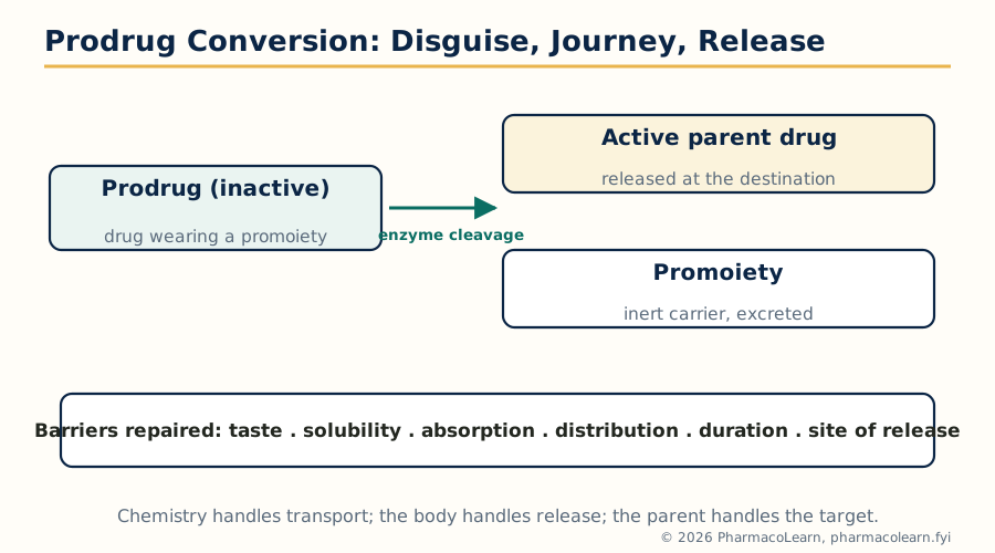 Figure: Prodrug conversion: the disguised drug makes the journey, the promoiety is cleaved, and the active parent drug is released at the destination.
5.10 Prodrugs to improve patient acceptability
A drug a patient refuses is a drug that fails. Acceptability prodrugs mask properties that make dosing unpleasant. The classical case is taste: chloramphenicol is intensely bitter, and its palmitate ester is essentially tasteless because it does not dissolve, and therefore is not tasted, in the mouth; intestinal enzymes hydrolyse it to the parent. The same logic reduces the pain of injections (an irritating parent presented as a bland ester in an oily depot), the odour or gastric irritation of others, and generally trades a formulation problem the patient experiences for a cleavage step the body performs silently.
5.11 Prodrugs to improve drug solubility
Insolubility defeats dosage forms, above all injections, which demand a true solution. The solubility prodrug attaches an ionizable, water loving promoiety, classically a phosphate ester, to the parent: the prodrug dissolves freely, is administered, and phosphatases in blood and tissues release the parent. Fosphenytoin, the phosphate prodrug of phenytoin, is the standard example: freely water soluble where phenytoin is not, it can be given intravenously or intramuscularly without the aggressive solvents and the tissue damage of the older formulation. Chloramphenicol sodium succinate plays the same role for parenteral chloramphenicol. The design constraint is conversion kinetics: cleavage must be fast and complete enough that dosing the prodrug is equivalent to dosing the parent, and the equivalence must be demonstrated, not assumed.
5.12 Prodrugs to improve absorption and distribution
More prodrugs exist for this goal than any other, because absorption is where lipophilicity earns its keep. The ester strategy raises membrane permeability by masking a polar, ionized group, then surrenders the ester to plasma and tissue esterases:
- Enalapril is the ethyl ester of enalaprilat; the parent diacid is too polar to absorb well, the ester crosses the gut, and hydrolysis in the liver releases the ACE inhibitor.
- Oseltamivir is the ethyl ester of its active carboxylate; the ester is absorbed, the acid is not, and the antiviral is delivered by the same trick.
- Valaciclovir couples valine to aciclovir so that an intestinal peptide transporter carries the prodrug across, multiplying the aciclovir exposure the parent achieves; here the promoiety recruits a transporter rather than merely hiding polarity.
- Levodopa solves a distribution problem: dopamine cannot cross the blood brain barrier, but levodopa, an amino acid, is carried across by the neutral amino acid transporter and decarboxylated to dopamine in the brain, the bioprecursor pattern of section 5.9 at its most famous.
Distribution prodrugs in general aim the parent at a tissue: increasing brain entry, prolonging residence, or, in the next section, releasing only at a chosen site.
5.13 Site specific delivery and sustained action through prodrugs
Site specific delivery arranges for conversion to happen at the target and nowhere else. Sulfasalazine is the textbook design: 5 aminosalicylic acid, the anti inflammatory active in ulcerative colitis, is joined by an azo bond to sulfapyridine; the intact molecule passes the upper gut largely unabsorbed, and colonic bacteria reduce the azo bond exactly where the disease is, releasing the active agent in the colon. Enzyme targeted strategies generalize the idea, exploiting enzymes enriched at the site (including, experimentally, antibody directed enzyme prodrug therapy in cancer, where an antibody delivers an activating enzyme to the tumour before the prodrug is given). Sustained action uses the opposite kinetic arrangement: the prodrug is built to convert slowly, so it acts as a chemical depot. Long chain fatty acid esters of antipsychotics such as fluphenazine decanoate, injected in oil, hydrolyse over weeks, converting a daily oral adherence problem into a monthly injection, the pharmacokinetic repair of a social problem.
PRODRUG DESIGN, DECISION FLOW

  Parent drug has a named barrier: taste? solubility?
  absorption? distribution? duration? site?
      |
      v
  Choose a promoiety that repairs that barrier
  and a bond the body can cleave (usually an ester)
      |
      v
  Check conversion: where, by what enzyme, how fast,
  and is the promoiety itself harmless?
      |
      v
  Check stability: shelf life in the bottle,
  survival to the conversion site
      |
      v
  The prodrug is a new drug: full testing follows
5.14 The rationale of prodrug design
The rationale assembles the preceding sections into one argument. Begin with a parent whose pharmacology is right and whose pharmaceutical or pharmacokinetic behaviour is wrong in a specific, nameable way; the prodrug is justified only when the defect is in delivery, not in the target interaction, since no promoiety repairs a weak pharmacophore. Choose the promoiety to remove exactly that defect and no more, because every addition changes solubility, stability and conversion together. Arrange conversion to occur at the intended site, at a rate matched to the dosing plan, by enzymes reliably present in patients. Then the prodrug is not a trick but a division of labour: chemistry handles transport, biology handles release, and the parent handles the target.
5.15 Practical considerations of prodrug design
The practical register closes the unit, and it is where elegant designs are audited:
- Conversion reliability: the activating enzymes vary between species, which has misled many animal based programmes, and between patients, through genetics, age, disease and interacting drugs; a prodrug activated by a variable enzyme inherits that variability as variable dosing.
- Promoiety safety: the released carrier is a chemical dose in its own right and must be innocuous at the exposure involved; history's cautionary examples come from promoieties, such as formaldehyde releasing groups, that were not as innocent as assumed.
- Stability balance: the bond must survive manufacture, shelf storage and the journey to the conversion site, yet cleave promptly on arrival; too stable and the drug passes through unconverted, too labile and it is a parent drug with extra steps.
- Incomplete conversion and competing pathways: if cleavage is partial, or metabolism diverts the prodrug elsewhere, exposure to the parent becomes unpredictable, and the programme must measure parent, not prodrug, as the active currency.
- Regulatory reality: a prodrug is a new chemical entity, requiring its own full characterization and safety evaluation; the shortcut it offers is pharmacological, not administrative.
Read with Unit 4, this closes the subject's arc: targets are found and validated, leads are found and measured, relationships are made quantitative and three dimensional, and where the winning molecule still cannot reach its target, chemistry disguises it for the journey.
Frequently Asked Questions
Q: What is the difference between target identification and target validation? Identification names a molecule that a drug could act on, based on its place in disease biology. Validation proves the harder claim: that modulating this molecule, in the right direction, will actually change the disease in a patient at tolerable cost. Evidence climbs a ladder from association, through human genetics and pharmacological and transgenic experiments, to clinical proof. Most costly discovery failures are validation failures: excellent chemistry against targets that turned out not to matter.
Q: A knockout mouse lacking the target shows no protection from disease. Is the target dead? Not automatically. A germline knockout removes the protein for the animal's whole development, and other pathways can compensate, masking a role that acute blockade would reveal; the protein may also matter only in one tissue or disease stage. The result weakens the target and demands a second test, an inducible or conditional knockout, knockdown by siRNA or antisense, or a tool compound, before the programme is killed. Validation is a weight of evidence, not a single experiment.
Q: Combinatorial chemistry and high throughput screening are often named together. How do they differ? They are the supply and the test of lead identification. Combinatorial chemistry manufactures large libraries of related compounds by combining building blocks systematically, by parallel synthesis or split and mix methods. High throughput screening tests large collections, from any source, against the assay, using robotics and miniaturized plates. One makes candidates at scale; the other interrogates candidates at scale; a library from combinatorial chemistry is one of the things HTS screens.
Q: When is homology modelling used, and when threading? Both predict protein structure from sequence. Homology modelling applies when a related protein of known structure exists: the target sequence is aligned to that template and the model is copied and adapted from it, with accuracy rising with sequence identity. Threading is the fallback when no sequence relative can be found: the sequence is fitted against a library of known folds and scored for compatibility, identifying the likely fold family but not atomic detail. Homology gives coordinates for design; threading gives architecture for triage.
Q: NMR and X-ray crystallography both determine protein structure. What decides between them? Crystallography needs the protein to crystallize, and then delivers high resolution structures, including drug complexes, at relatively high throughput; most structures used in design come from it. NMR works in solution, needs no crystals, reports conformational dynamics, and can detect weak ligand binding directly, but is limited to smaller proteins and is slow and expert intensive. They are complements: crystallography for the design cycle, NMR for solution behaviour, small domains and binding studies.
Q: What, in one sentence each, is the core difference between traditional and rational drug design? Traditional design finds a molecule by its effect in a whole system first and learns its mechanism later, if ever: effect before explanation. Rational design starts from knowledge of the disease mechanism and the target, designs the molecule to fit that knowledge, and tests the stated hypothesis: explanation before effect. Modern programmes are hybrids, rational in choosing the target and assay, empirical in running screens, rational again in optimizing what the screens return.
Q: Is Lipinski's rule of five a law that a drug must obey? No. It is a statistical screen distilled from marketed oral drugs: absorption and permeation problems become more likely beyond molecular weight 500, log P 5, 5 hydrogen bond donors and 10 acceptors. In drug likeness screening it flags risk, one violation warning and two arguing against a series, but genuine drugs violate it, notably natural products, non oral drugs and transporter substrates. Deleting every violator would delete real medicines; ignoring it entirely fills pipelines with large, greasy failures.
Q: Rigid, flexible and manual docking: what changes between them? The amount of motion allowed in the search. Rigid docking moves a fixed ligand conformation through the site as one body: fastest, and it misses poses that need the ligand to bend. Flexible docking explores the ligand's rotatable bonds during placement, usually with the protein held rigid or nearly so, and is the standard working method. Manual docking is placement by a scientist at a graphics screen, slowest of all, used to build and inspect hypotheses for the few compounds that matter most. Speed falls and realism rises along the series.
Q: Hansch and Free Wilson analysis both predict activity. When is each preferred? Hansch analysis relates activity to physicochemical parameters (log P, sigma, steric terms) of the substituents, so it can estimate a substituent never yet made and it reveals an optimum, such as the best log P. It needs parameter values and a single mechanism across the series. Free Wilson analysis uses only the series' own data, adding each substituent's measured contribution to the parent activity, so it needs no property assumptions but can only recombine substituents already synthesized, and fails where substituents interact. Fujita's mixed approach combines the two where each is strongest.
Q: Why would a designer deliberately make an inactive molecule, a prodrug? Because the active molecule often cannot complete the journey: too insoluble to inject, too polar to absorb, too bitter to swallow, excluded from the brain, or gone in hours. The prodrug is the active drug in a temporary disguise chosen to repair that one delivery defect: enalapril's ester gets the ACE inhibitor absorbed, levodopa's amino acid form gets dopamine's precursor into the brain, sulfasalazine's azo bond holds release until the colon. Body enzymes remove the disguise at the destination, and the freed parent does the pharmacology.
Complete MPL203T notes, all 5 units in one PDF, free to keep.
Other M.Pharm subjects: MPH101T · MPC101T · MPL101T · MPH102T · MPH103T · MPH104T · MPL102T · MPL103T · MPL104T · MPC102T · MPC103T · MPC104T · MPH201T · MPH202T · MPH203T · MPH204T · MPC201T · MPC202T · MPC203T · MPC204T · MPL201T · MPL202T · MPL203T · MPL204T · MRA101T · MRA102T · MRA103T · MRA104T · MRM301T · MPG101T · MPG102T · MPG103T · MPG201T · MPG202T · MPG203T · MPG104T · MPG204T · MRA201T · MRA202T · MRA203T · MRA204T · M.Pharm