
MPH203T — Computer Aided Drug Delivery System
4 hrs/week, 4 credits, 60 hours, 100 marks (75 end semester + 25 sessional). Notes follow the M.Pharm syllabus, unit by unit.
MPH203T Computer Aided Drug Delivery System notes for M.Pharm Semester 2 Pharmaceutics: statistical modelling and QbD, modelling of drug disposition and transporters, factorial design and optimization, GI absorption simulation, AI, robotics and CFD, with free unit wise PDF downloads on PharmacoLearn.
Units in this subject
- Unit 1 — Computers in Pharmaceutical Research and Development: A General Overview; Quality-by-Design in Pharmaceutical Development
- Unit 2 — Computational Modeling of Drug Disposition
- Unit 3 — Computer-aided formulation development
- Unit 4 — Computer-aided biopharmaceutical characterization; Computer Simulations in Pharmacokinetics and Pharmacodynamics; Computers in Clinical Development
- Unit 5 — Artificial Intelligence (AI), Robotics and Computational fluid dynamics
Download MPH203T PDF Notes
Free PDFs for this subject, one per unit:
Computer Aided Drug Delivery System, subject code MPH203T, is a core Semester 2 subject of M.Pharm Pharmaceutics. It carries 4 credits and 60 hours of theory, taught at 4 hours per week, for 100 marks.
The computer has moved from the edge of pharmaceutical work to its centre. Almost every decision in modern drug development, which molecule to advance, which formulation to scale up, which dose to take into patients, is now made first on a screen and only then at the bench. This subject follows that idea through the whole research and development process. The first unit starts with how computers entered pharmaceutical research, the statistical modelling that underlies all later units (descriptive and mechanistic models, estimation, confidence regions, sensitivity analysis, optimal design and population modelling), and Quality by Design, the ICH Q8 framework that turned modelling and designed experiments into a regulatory expectation. The second unit models what the body does to the drug: computational prediction of absorption, solubility, intestinal permeation, distribution and excretion, with the active transporters (P-gp, BCRP, hPEPT1, ASBT, OCT, OATP, the nucleoside and blood brain barrier choline transporters) that decide the fate of many molecules. The third unit applies computers to the formulation itself: the concept of optimization, factorial and screening designs, the computer aided development of emulsions and microemulsion carriers, and the legal, ethical and commercial frame (protection of computer based innovation, ethics of computing, market analysis). The fourth unit simulates the dosage form in the body: gastrointestinal absorption simulation with model construction, parameter sensitivity analysis, virtual trials and fed versus fasted prediction, the link to dissolution and IVIVC and biowaivers, simulations in pharmacokinetics and pharmacodynamics from the whole organism down to genes, and computers in clinical development, including clinical data management and the regulation of computer systems. The last unit looks at the newest tools: artificial intelligence, robotics and pharmaceutical automation, and computational fluid dynamics, with their applications, advantages, disadvantages and future directions.
Unit 1: Computers in Pharmaceutical Research and Development and Quality by Design
1.1 History of computers in pharmaceutical research and development
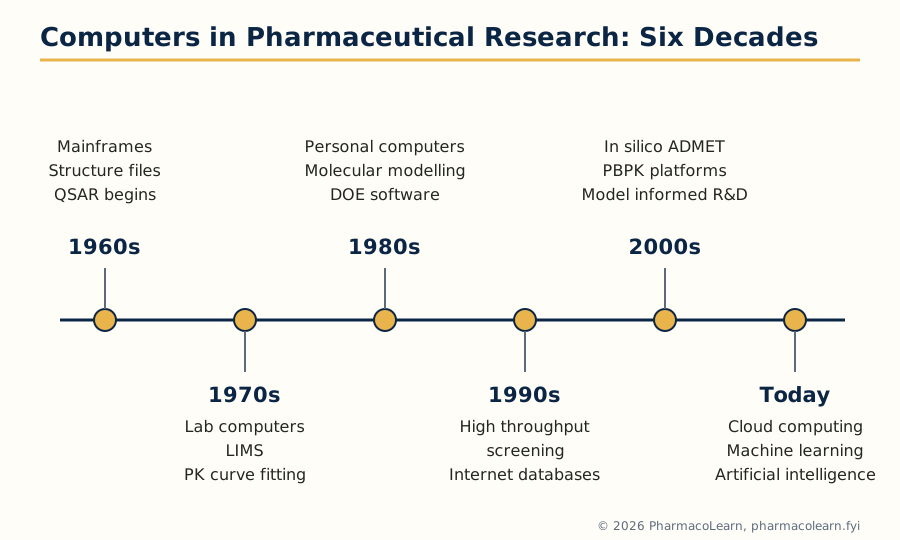 Figure: Sixty years of computing in pharmaceutical research. Each decade first automated a manual task, then made a previously impossible task routine.
Computers entered pharmaceutical research in the 1960s, when mainframe machines were first used to store chemical structure files, search compound collections and process the growing volume of analytical and pharmacological data that manual records could no longer handle. The same decade produced the first genuinely computational science of the field: quantitative structure activity relationships (QSAR), in which Hansch and others showed that biological activity could be regressed against computed physicochemical descriptors such as partition coefficients and electronic parameters. In the 1970s, laboratory minicomputers took over instrument control and data capture, laboratory information management systems (LIMS) began to organise samples and results, and pharmacokinetic curve fitting moved from graph paper to nonlinear regression programs. The 1980s brought the personal computer and the graphics workstation: molecular modelling and docking became visual, interactive activities, spreadsheets entered the formulation laboratory, and statistical packages made designed experiments practical for ordinary development teams. The 1990s were the decade of scale: combinatorial chemistry and high throughput screening generated data faster than scientists could inspect it, the internet connected databases and collaborators, and bioinformatics grew up alongside the sequencing of genomes. In the 2000s the emphasis shifted from generating data to predicting outcomes: in silico ADMET screening, physiologically based pharmacokinetic (PBPK) platforms and the first regulatory acceptance of modelling and simulation as formal evidence, including the United States Food and Drug Administration (US FDA) promoting model informed drug development. The pattern across six decades is constant: each generation of hardware first automated an existing manual task, then made a previously impossible task routine.
1.2 Computers in pharmaceutical research: a general overview
Read as a map, this subject is the tour of a single idea, the computer as a decision tool, applied at every stage of research and development. In discovery, computers screen virtual libraries, predict activity and filter out molecules with hopeless solubility, permeability or toxicity before synthesis. In preclinical development they model drug disposition (Unit 2), so that animal and early human studies are designed around predicted behaviour instead of discovered surprises. In formulation development they replace one factor at a time tinkering with designed experiments and optimization (Unit 3). In biopharmaceutical evaluation they simulate the dosage form in a virtual gut and a virtual population (Unit 4), linking dissolution to plasma profiles and supporting biowaiver arguments. In clinical development they capture, clean and lock trial data and keep the systems that hold them compliant (Unit 4). Two threads run through all of it: every computer method in the list is a model, a simplified mathematical stand in for a real system, and every model must be built, checked and used within its limits. The statistical modelling of the rest of this unit is the grammar for all of that.
1.3 Statistical modeling in pharmaceutical research: descriptive versus mechanistic modeling
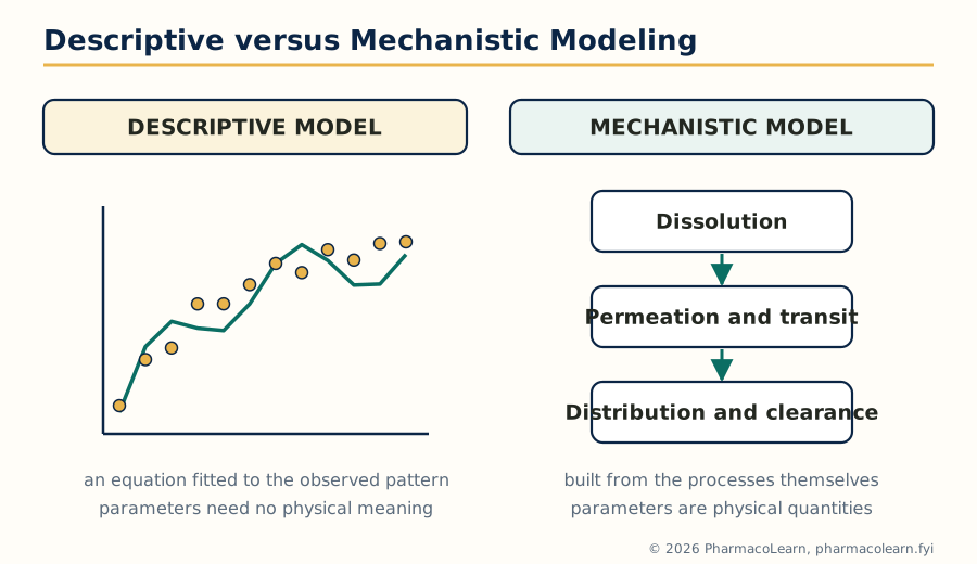 Figure: The two modelling philosophies of Unit 1. The descriptive model follows the data; the mechanistic model follows the process, and can therefore be extrapolated with stated assumptions.
A statistical model is an equation, with parameters, that connects inputs (dose, formulation variables, patient properties) to outputs (concentrations, responses, quality attributes) and leaves a residual for what it cannot explain. The syllabus divides modelling into two philosophies. A descriptive (empirical) model describes the pattern in the data without claiming to represent the underlying process: a polynomial fitted to a dissolution profile, or a compartment model used simply because its curve matches the plasma data. Its parameters need have no physical meaning, it is cheap to build, and it usually interpolates well inside the studied range, but it cannot be trusted outside that range, because nothing in it knows why the data bend the way they do. A mechanistic model is built from the actual processes believed to generate the data: dissolution, permeation and transit compartments for absorption (Unit 4), enzyme kinetics for metabolism, receptor binding for effect. Its parameters are physical quantities (a permeability, a clearance, a rate constant), it can extrapolate with some justification to new doses, formulations and populations, and it can be falsified process by process when it fails. The price is that it needs more knowledge, more parameters and more data to support them. Practice uses both, often in sequence: a descriptive model early, when little is known, and a mechanistic model when the programme is mature enough to ask "what if" questions.
| Feature | Descriptive (empirical) model | Mechanistic model |
|---|---|---|
| Basis | Pattern in the observed data | The physical and biological processes generating the data |
| Parameters | Curve fitting constants, often without physical meaning | Physical quantities: permeability, clearance, rate constants |
| Data needed | The dataset being described | Process knowledge plus data to estimate the physical parameters |
| Interpolation | Usually good inside the studied range | Good, and structured by the process |
| Extrapolation | Unsafe outside the studied range | Possible with stated assumptions, and testable |
| Typical examples | Polynomial fit to a dissolution profile; empirical PK curve fit | PBPK model; ACAT gastrointestinal absorption model; receptor occupancy PD model |
1.4 Statistical parameters and estimation
Every model carries parameters: the fixed numbers that must be learned from data before the model can predict anything, such as the slope and intercept of a calibration line, the elimination rate constant and volume of a compartment model, or the coefficients of a factorial design equation (Unit 3). Estimation is the statistical procedure that chooses parameter values making the model agree best with the observations. Two estimation principles dominate pharmaceutical work. Least squares chooses the values that minimise the sum of squared differences (residuals) between observed and predicted values; weighted least squares gives less influence to less precise observations, which matters for concentration data whose error grows with the value. Maximum likelihood chooses the values under which the observed data are most probable, given an assumed error distribution, and is the engine inside population modelling software (section 1.9). Estimated parameters are never exact: each carries uncertainty, expressed as a standard error, and a fit must be judged not by whether the curve touches the points but by whether the residuals are patternless, the parameters are estimated with usable precision, and the model predicts new data.
1.5 Confidence regions
Because parameters are estimated from finite, noisy data, a point estimate is only half an answer. A confidence interval gives the range of values for one parameter compatible with the data at a stated confidence level, conventionally 95 percent: loosely, the range within which the true value is believed to lie, given the data and the model. When several parameters are estimated together, the corresponding object is a confidence region, a joint region in parameter space (an ellipse for two parameters, a volume for more). Regions matter because estimated parameters are usually correlated: raising one estimate can be compensated by lowering another while the fit barely changes, so two parameters can each look precise alone yet be poorly determined together, a warning sign in any model used for decisions. Narrow regions come from informative data, good designs (next sections) and models no more complex than the question requires.
1.6 Nonlinearity at the optimum
Much pharmaceutical optimization searches for an optimum: the formulation, dose or set of conditions giving the best response. Real response surfaces are curved, and near an optimum they are at their most curved, because a maximum or minimum is by definition where the surface bends over. This is the problem of nonlinearity at the optimum. Linear approximations, which are adequate on the flank of a surface, fail at the top: the estimated optimum position becomes uncertain, small parameter changes move the predicted optimum a long way, and the confidence region around the optimum is asymmetric and larger than linear theory suggests. Practical consequences follow. An optimum found by fitting should be confirmed by experiment at and around the predicted point, not trusted from the equation alone. Optimization should report not just the best point but the region of near optimal conditions, which is exactly the idea the design space of Quality by Design formalises (section 1.10). And where two very different settings give nearly equal responses, the flatter, more robust one is usually the better manufacturing choice.
1.7 Sensitivity analysis
Sensitivity analysis asks how much a model's output changes when its inputs or parameters change. It is the standard way of finding out what a model actually depends on. In the local form, one parameter at a time is varied by a small amount around its estimate while the others are held fixed, and the resulting change in output (a plasma concentration, a predicted response, a quality attribute) is recorded, often drawn as a ranked bar or tornado chart. In the global form, all parameters are varied together across their plausible ranges, typically by simulation, so interactions between parameters are captured as well. A prediction whose output is violently sensitive to a parameter nobody has measured is not a prediction but a guess, and sensitivity analysis is how that is found out before the clinic does it.
1.8 Optimal design
If sensitivity analysis asks what a model depends on, optimal design asks how an experiment should be run so that the model is estimated as well as possible. Classical designs (Unit 3) spread experimental runs by habit and symmetry. Optimal design instead starts from the model and a criterion: choose the experimental conditions, the sampling times, doses or factor settings, that maximise the information the data will carry about the parameters. The machinery is the Fisher information matrix, which summarises how precisely the parameters can be estimated from a given design; the most used criterion, D-optimality, chooses the design that maximises the determinant of that matrix, equivalently minimising the volume of the joint confidence region of the parameters. Optimal design is used heavily in pharmacokinetics, where it answers questions such as the few best blood sampling times for estimating clearance and volume in a trial that can afford only sparse samples in each patient, and in formulation work, where it can build a small, efficient design for an awkward factor space that no textbook design fits. Its weakness mirrors its strength: the optimal design is optimal for the assumed model and parameter values, so sound practice checks the design across plausible parameter values and keeps some robustness in reserve.
1.9 Population modeling
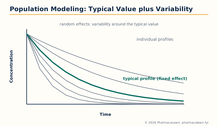 Figure: Population modeling in one picture: every subject has a profile, the model estimates the typical profile and the distribution of variability around it, explained and unexplained.
Classical pharmacokinetic analysis fits one subject at a time. Population modeling fits all subjects at once with a model that has two levels: fixed effects, the typical parameter values and the systematic influence of patient properties (covariates) such as weight, age, renal function and genotype; and random effects, the unexplained variability between subjects and the residual variability within a subject over time. The result is not just an average curve but a description of the whole distribution of behaviour in the population, including how much of the variability is explained by measurable covariates. This matters because drug development decisions are population decisions: a dose must work across patients, including the slow metaboliser and the patient with poor kidneys, not just in the average volunteer. Population modelling handles the sparse, unbalanced data that real trials produce (a few samples per patient, at different times), where one subject at a time fitting is impossible, and it is the standard analysis behind dose recommendations in special populations. The approach was pioneered in the NONMEM software tradition, in which the model is written as differential equations for the typical individual plus statistical models for variability, and estimated by likelihood based methods (section 1.4). The same two level thinking, typical value plus structured variability, underlies the virtual trials of Unit 4.
1.10 Quality by Design in pharmaceutical development: introduction and ICH Q8
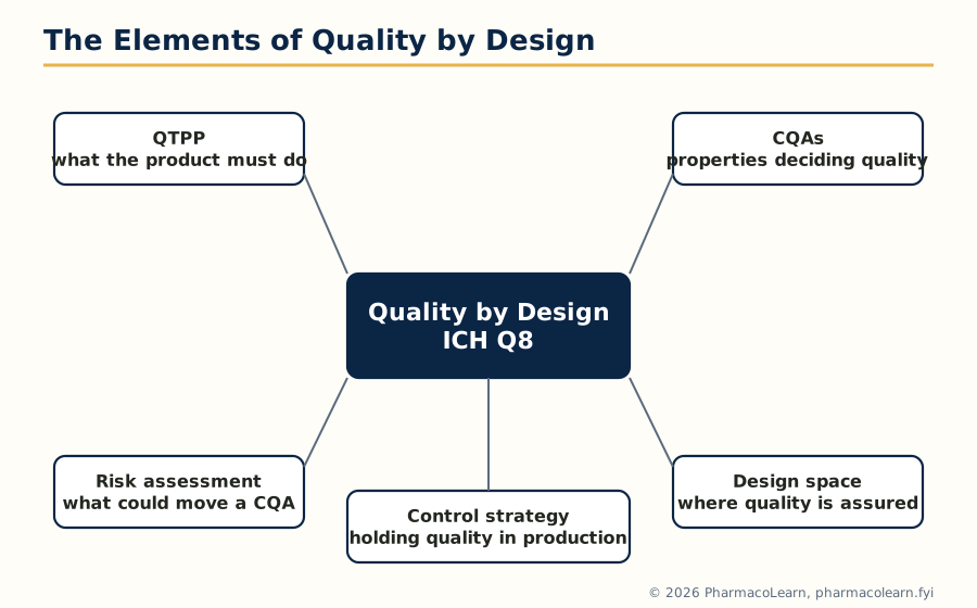 Figure: The elements of Quality by Design under ICH Q8. The QTPP states the goal, CQAs define quality, risk assessment ranks the dangers, the design space marks where quality is assured, and the control strategy holds production inside it.
Quality by Design (QbD) is the systematic approach to development that begins with predefined objectives and emphasises product and process understanding and process control, based on sound science and quality risk management. That definition is from ICH Q8, the International Council for Harmonisation guideline on pharmaceutical development, which is the regulatory core of this topic (the current version, ICH Q8(R2), is read together with ICH Q9 on quality risk management and ICH Q10 on the pharmaceutical quality system). QbD replaced the older quality by testing philosophy, in which quality was verified at the end by testing the finished batch, with the principle that quality should be built in by understanding. Its working elements are:
- Quality target product profile (QTPP): a prospective summary of the quality characteristics the product should have to ensure the desired clinical performance: dosage form, route, strength, release profile, stability and the attributes patients and clinicians depend on.
- Critical quality attributes (CQAs): the physical, chemical, biological or microbiological properties that must lie within limits to ensure the desired quality, for a tablet typically assay, content uniformity, dissolution and degradation products.
- Risk assessment: structured tools (cause and effect diagrams, failure mode and effects analysis) linking material attributes and process parameters to CQAs and ranking what matters, so effort goes where risk is.
- Critical material attributes and critical process parameters: the input variables whose variation moves a CQA, identified from the risk assessment and from prior knowledge.
- Design space: the multidimensional combination and interaction of input variables and process parameters that has been demonstrated to provide assurance of quality. Working within the design space is not considered a change by regulators; moving outside it is.
- Control strategy: the planned set of controls, on materials, process conditions, in process measurements and finished product testing, that together ensure the process performs and the product meets its CQAs, maintained across the product lifecycle with continual improvement.
| QbD element | What it answers | Typical output for a tablet |
|---|---|---|
| QTPP | What must the product do? | Immediate release tablet, stated strength, dissolution target, 24 month shelf life |
| CQA | Which properties decide quality? | Assay, content uniformity, dissolution, impurities |
| Risk assessment | What could move a CQA? | Ranked list: granulation moisture and compression force ranked high |
| Design space | Where is quality assured? | A region of moisture, force and speed combinations proven acceptable |
| Control strategy | How is quality held in routine production? | Material specifications, in process controls, PAT checks, end product tests |
1.11 Regulatory and industry views on QbD
Regulators and industry arrived at QbD from opposite frustrations. For regulators, the quality by testing system produced products that passed their specifications yet were made by processes nobody fully understood, so any manufacturing change demanded fresh regulatory submissions and approval delays, discouraging improvement. The US FDA's process analytical technology (PAT) initiative and the ICH Q8, Q9 and Q10 guidelines reframed the bargain: a manufacturer who demonstrates genuine process understanding, through risk assessment, designed experiments and a design space, earns regulatory flexibility, including movement within the approved design space without prior approval, and a science and risk based review. The European Medicines Agency holds the same position, and joint FDA and EMA question and answer documents exist precisely because both agencies review QbD applications. Industry's view is the mirror image: QbD development costs more at the start (more experiments, more modelling, more documentation) and pays back across the lifecycle, in fewer failed batches and out of specification results, smoother scale up and technology transfer, faster handling of changes, and a process that stays in control because its behaviour is understood rather than merely observed.
1.12 Scientifically based QbD: examples of application
A scientifically based QbD study is the practical union of this whole unit, so one worked pattern is worth following. Consider an immediate release tablet programme. The QTPP is written first, with the dissolution target the clinical team needs. Prior knowledge and a risk assessment identify the plausible critical variables: granulation moisture, lubricant level and blending time, and compression force, acting on the CQAs of dissolution, hardness related handling quality and content uniformity. A screening design (Unit 3) tests many candidate variables in few runs and keeps the vital few. A factorial or response surface design then maps the survivors, fitting a mechanistic leaning statistical model of dissolution and uniformity against the variables; sensitivity analysis (section 1.7) confirms which effects dominate; confidence regions (section 1.5) show how firmly the boundaries are known; and the design space is declared as the region where the model, with its uncertainty, predicts all CQAs in specification with high probability. Routine manufacture then runs under a control strategy that may include PAT monitoring of granulation, and the knowledge is filed so that post approval movement inside the space is a quality system action, not a new licence application. The same pattern, varying only the product, is reported in the literature for modified release tablets, lyophilised products and biological processes: define the target, assess risk, design experiments, model, define the space, control it, and keep learning across the lifecycle.
The QbD workflow of ICH Q8
QTPP: what the product must do
   |
   v
CQAs: the properties that decide quality
   |
   v
Risk assessment: rank materials and parameters
   |
   v
Designed experiments and models (Units 1 and 3)
   |
   v
Design space: where quality is assured
   |
   v
Control strategy and lifecycle learning
Unit 2: Computational Modeling of Drug Disposition
2.1 Introduction: why disposition is modeled
Disposition is what happens to a drug after it reaches the body: absorption into the circulation, distribution to the tissues, and excretion or metabolism out of them (the ADME sequence, with metabolism usually counted alongside). Every step can lose the drug, delay it or concentrate it in the wrong place, and historically each was discovered experimentally, late and expensively, in animal studies or in failed clinical trials. Computational modeling of drug disposition exists to move that discovery earlier and cheaper: to predict, from chemical structure and a modest set of laboratory measurements, how a molecule will be absorbed, where it will go, how long it will stay and how it will leave, before large studies begin. The predictions prioritise which molecules deserve synthesis and testing, design the experiments that follow (doses, sampling times, species), and flag the liabilities, poor solubility, efflux by transporters, rapid clearance, that formulation scientists (MPH201T, MPH202T) will have to engineer around. The methods range from structure based statistical predictions that need nothing but the molecule's drawing, to full physiological simulations (Unit 4) that need measured data. This unit takes the modeling techniques step by step along the disposition pathway, and ends with the active transporters, the membrane proteins that the syllabus names individually because they defeat simple predictions and must be modeled explicitly.
2.2 Modeling techniques: the levels of modeling
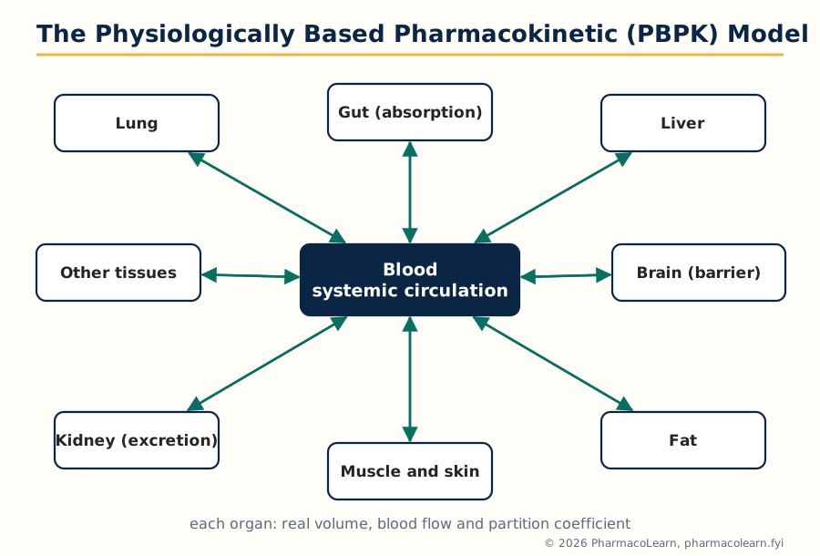 Figure: The physiologically based pharmacokinetic model. Organs are real compartments with volumes and blood flows, joined by the circulation; the drug's physicochemical and in vitro properties decide how it partitions into each.
Three families of technique cover the field. Structure based (in silico) prediction computes or correlates properties from the molecular structure itself: calculated descriptors such as molecular weight, partition coefficient (log P), polar surface area, hydrogen bond donors and acceptors, and rotatable bonds feed statistical (QSAR type) models trained on measured data for solubility, permeability and activity. Simple rule sets, of which the Lipinski criteria (molecular weight not above 500, log P not above 5, limited hydrogen bonding) are the famous example, act as early filters for oral drug likeness. Compartmental modeling treats the body as a small number of well mixed pools connected by first order transfers (MPH202T, Unit 3): empirical, data driven, excellent for describing and interpolating measured concentration profiles, weaker for predicting a new molecule. Physiologically based pharmacokinetic (PBPK) modeling builds the body from organs and tissues with real volumes and blood flows, and the drug's movement from its physicochemical and in vitro properties: mechanistic (section 1.3), more demanding, but able to predict a profile before any human data exist and to extrapolate across doses, populations and formulations. Modern disposition modeling chains the three: structure based predictions feed the PBPK model, the PBPK model predicts the profile, and compartmental or population analysis (section 1.9) refines parameters once data arrive.
2.3 Modeling drug absorption
Absorption modeling predicts the rate and extent to which an oral dose reaches the portal blood. A complete absorption model multiplies two chances: the drug must dissolve in the gut fluids, and the dissolved drug must cross the intestinal wall, while both processes race against transit out of the absorbing region. Inputs are the drug's solubility (section 2.4), its permeability (section 2.5), dose and particle or formulation properties, and gut physiology: regional pH, fluid volumes, transit times and surface areas. Models range from simple classifications, the biopharmaceutics classification system (BCS) sorting drugs by solubility and permeability into four classes that predict whether dissolution or permeation limits absorption, to the full gastrointestinal simulation of Unit 4, which follows the dose compartment by compartment. Outputs are the fraction absorbed, and with distribution and clearance added, the predicted plasma profile including Cmax and Tmax. The formulator uses the same model in reverse: if dissolution limits absorption, particle size reduction or a solubility enhancing formulation is the fix; if permeation limits it, no amount of dissolution improvement will help, which is precisely the kind of decision the modeling exists to support.
2.4 Modeling solubility
Solubility decides how much drug can be in solution at once, and so caps the absorption rate. Computational work addresses two quantities. Intrinsic solubility is the solubility of the unionised molecule, predictable in silico from structure by models trained on measured values, using descriptors that capture crystal packing (melting point is a practical surrogate: a high melting, strongly crystalline solid is usually a poorly soluble one) and solvation. pH dependent solubility follows from the intrinsic value and the pKa by the Henderson-Hasselbalch relations worked in MPH202T: solubility rises as ionisation rises, steeply for strong acids and bases, so a weak base may be freely soluble in the stomach and nearly insoluble in the intestine, with the risk of precipitation on transit, a phenomenon the Unit 4 simulation tracks explicitly. Measured solubility in biorelevant media (simulated gastric and intestinal fluids, including bile salt media for the fed state) anchors the models, and the modelling of solubility is also where salt selection, polymorph screening and amorphous strategies are compared on paper before they are compared in the laboratory. The honest limit is accuracy: in silico solubility predictions are commonly within about half to one log unit of measurement, good enough to rank compounds, not good enough to replace measuring the candidates that matter.
2.5 Modeling intestinal permeation
Permeation is the crossing of the intestinal wall by dissolved drug. Experimentally it is measured in cell monolayers, the Caco-2 human intestinal cell line above all, and in artificial membrane systems (PAMPA) that isolate passive diffusion, and the modeling task is to predict the human effective permeability from such data or from structure. In silico models use the same descriptor family as solubility models: lipophilicity raises passive permeation, while size, charge and hydrogen bonding capacity lower it, so permeation and solubility pull in opposite directions on lipophilicity, which is why drug design is a compromise. Permeation models must also decide whether the molecule merely diffuses or is carried: uptake and efflux transporters (sections 2.8 to 2.13) make measured permeability direction dependent, with an efflux ratio between the two directions across a cell layer as the standard experimental signal that a transporter is involved. A modeled permeability then enters the absorption model of section 2.3 and the gastrointestinal simulation of Unit 4, where it competes with dissolution and transit to set the fraction absorbed.
2.6 Modeling drug distribution
Distribution modeling predicts where the drug goes after absorption: the volume of distribution at its simplest, and in PBPK work a concentration in each tissue. The governing idea is partitioning: drug moves between blood and tissue until the unbound concentrations equalise, so tissue levels are set by tissue composition (water, lipid, protein) and the drug's binding and lipophilicity. PBPK models compute tissue to plasma partition coefficients from composition based equations using the drug's log P, pKa, fraction unbound in plasma and blood to plasma ratio, all measurable or predictable in vitro. Plasma protein binding is itself modeled and measured, because only unbound drug distributes, acts and is cleared, and binding displacement is a classic interaction mechanism (MPH202T, Unit 3). Distribution modeling also handles the barriers: the blood brain barrier as a distribution problem with tight junctions and efflux transporters (section 2.13), the placenta, and sanctuaries such as the eye.
2.7 Modeling drug excretion
Excretion removes drug, unchanged or as metabolites, through the kidney and the bile. Renal excretion modeling starts from the three kidney processes: glomerular filtration, which passes unbound drug and is predicted well from the fraction unbound and the glomerular filtration rate; active tubular secretion, carried by transporters (section 2.12) and much harder to predict; and tubular reabsorption, which returns lipophilic unionised drug to the blood and is therefore pH and urine flow dependent, the basis of urine alkalinisation in salicylate poisoning. Biliary excretion moves drug from hepatocytes into bile through canalicular efflux transporters, favoured by larger, amphiphilic molecules, and connects to the enterohepatic recycling of section 2.11 when the excreted drug or its conjugate is reabsorbed from the gut. In PBPK practice, total clearance is assembled from such organ clearances plus metabolism, and excretion modeling is what allows predictions for patients with renal impairment, a population in which doses must fall with filtration, and for transporter mediated interactions at the kidney and liver.
2.8 Active transport: the transporters as gatekeepers
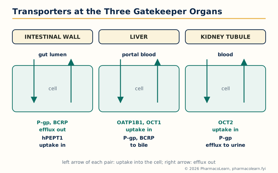 Figure: Uptake and efflux transporters at the three gatekeeper organs. Disposition at each barrier is the balance of the two directions, which is why transporters are modeled explicitly.
Passive diffusion is only half the membrane story. Membrane transporter proteins move specific substrates across cell membranes, uphill if necessary, and organs place them exactly where disposition is decided: the intestinal wall, the liver, the kidney tubule and the blood brain barrier. Transporters divide by direction of effect. Efflux transporters of the ATP binding cassette (ABC) family, powered by ATP, pump substrates out of cells: into the gut lumen, into bile, into urine, or back into blood at the brain. Uptake transporters of the solute carrier (SLC) family carry substrates into cells: from gut lumen into enterocyte, from blood into hepatocyte, from filtrate back into blood. A drug that is a substrate of an efflux transporter may be poorly absorbed and excluded from the brain however good its passive permeability; a drug needing an uptake transporter to enter the liver may fail to be cleared, or to act, when that transporter is inhibited or genetically deficient. Modeling disposition therefore includes a transporter layer: which transporters accept the drug, where they sit, how strongly they act, and what happens when another drug inhibits them, the machinery behind a large share of modern drug drug interaction prediction. The syllabus names the principal players; the next sections take them in turn.
| Transporter | Family and direction | Main sites | Representative substrates or roles |
|---|---|---|---|
| P-gp (ABCB1) | ABC efflux | Gut wall, liver canaliculi, kidney, blood brain barrier | Digoxin, many anticancer drugs, ciclosporin |
| BCRP (ABCG2) | ABC efflux | Gut wall, liver, blood brain barrier, placenta | Rosuvastatin, sulfasalazine, topotecan |
| hPEPT1 (SLC15A1) | SLC uptake | Intestinal wall (apical) | Beta-lactam antibiotics, valaciclovir |
| Nucleoside transporters (CNT, ENT) | SLC uptake and equilibrative | Gut, liver, kidney, most tissues | Nucleoside analogue drugs: gemcitabine, zidovudine |
| ASBT (SLC10A2) | SLC uptake | Terminal ileum (apical) | Bile acids, enterohepatic recycling |
| OCT (SLC22A) | SLC uptake | Liver (OCT1), kidney (OCT2) | Metformin, cimetidine |
| OATP (SLCO) | SLC uptake | Liver (OATP1B1, OATP1B3), blood brain barrier | Statins, methotrexate, bilirubin |
| BBB choline transporter | SLC uptake | Blood brain barrier | Choline, for acetylcholine synthesis in brain |
2.9 P-glycoprotein and BCRP: the efflux pumps
P-glycoprotein (P-gp, gene ABCB1) is the best studied efflux transporter: a broad specificity pump in the apical membrane of enterocytes that ejects absorbed drug back into the gut lumen, in the canalicular membrane of hepatocytes ejecting drug into bile, in kidney tubule cells into urine, and in the endothelial cells of the blood brain barrier ejecting drug back into blood. Its modelling significance is threefold. In absorption, P-gp works with the enzyme CYP3A4 in the gut wall as a combined barrier, the pump repeatedly presenting the drug to the enzyme. In distribution, P-gp at the blood brain barrier is the reason many peripherally intended drugs spare the brain, and why the classic substrate digoxin, normally excluded, becomes neurotoxic when P-gp is inhibited. In interactions, P-gp inhibitors raise, and inducers lower, the plasma levels of substrate drugs, an effect PBPK models now predict quantitatively. Breast cancer resistance protein (BCRP, gene ABCG2), named from its discovery in resistant tumour cells, is the second great efflux pump, sharing many sites with P-gp and adding the placenta and the lactating mammary gland; its standard probe substrate is the statin rosuvastatin, whose exposure rises markedly when BCRP is inhibited or genetically reduced.
2.10 hPEPT1 and the nucleoside transporters: uptake into the body
The intestinal peptide transporter hPEPT1 (gene SLC15A1) moves dipeptides and tripeptides from the diet across the apical membrane of the enterocyte, and its broad specificity is a gift to drug design: molecules built to look like peptides are carried with it. Beta-lactam antibiotics such as cephalexin are substrates, and the prodrug strategy that defines this transporter is valaciclovir, the valine ester of aciclovir, which hPEPT1 carries so efficiently that the oral bioavailability of aciclovir rises several fold. Absorption models for such drugs must include the carrier: uptake is saturable, so fraction absorbed can fall as dose rises, and subject to competition between substrates. The nucleoside transporters handle the building blocks of DNA and RNA and, unavoidably, nucleoside analogue drugs. The concentrative nucleoside transporters (CNT family) use the sodium gradient to move nucleosides uphill into cells; the equilibrative transporters (ENT family) let them move down their gradient in either direction. Antiviral and anticancer nucleoside analogues, zidovudine and gemcitabine among them, depend on these carriers for cell entry, gemcitabine uptake through hENT1 being a studied determinant of its activity, and transporter expression in a tissue can decide whether the analogue reaches its intracellular target at all.
2.11 ASBT and enterohepatic recycling
The apical sodium dependent bile acid transporter (ASBT, gene SLC10A2) sits in the terminal ileum and reclaims bile acids from the gut lumen into the enterocyte, from where they return through the portal blood to the liver, the enterohepatic circulation that recycles the bile acid pool many times a day. Its place in disposition modeling is that anything riding this circuit, bile acids themselves, drugs excreted into bile and their conjugates hydrolysed by gut bacteria, can be reabsorbed rather than lost, producing long apparent half lives and sometimes secondary peaks in the plasma profile. A model that ignores recycling will underpredict exposure and misread the profile shape. ASBT is also a drug target in its own right, inhibitors interrupting the circuit to lower cholesterol or treat bile acid diarrhoea, and a potential delivery route for bile acid conjugated drugs aimed at the liver.
2.12 OCT and OATP: transporters of liver and kidney
The organic cation transporters (OCTs, gene family SLC22A) move small positively charged molecules into cells. OCT1 in the liver takes up cationic drugs from portal blood, and OCT2 in the kidney takes them up from blood into tubule cells for secretion into urine. Their textbook substrate is metformin: hepatic OCT1 governs its delivery to its site of action, renal OCT2 begins its dominant elimination route, and inhibitors such as cimetidine, itself an OCT2 substrate, raise metformin levels by blocking the renal step, a transporter interaction with no enzyme involved. The organic anion transporting polypeptides (OATPs, gene family SLCO) are uptake transporters of the liver above all: OATP1B1 and OATP1B3 sit on the blood facing membrane of hepatocytes and pull a wide range of anionic and neutral drugs, the statins prominently, out of blood into the liver for metabolism and biliary excretion. When OATP1B1 is inhibited, for example by ciclosporin, statin plasma levels climb and muscle toxicity risk follows; when its gene carries the reduced function variant common in the population, simvastatin exposure rises in carriers, one of the clearest pharmacogenetic findings in practice. PBPK models therefore carry OATP mediated hepatic uptake as an explicit, saturable, inhibitable step rather than burying it in a passive clearance term.
2.13 The BBB choline transporter
The blood brain barrier (BBB) is built to keep things out, tight junctions sealing its endothelium and efflux pumps (section 2.9) ejecting what diffuses in, yet the brain must import nutrients, and each nutrient carrier is a potential door for drugs. The BBB choline transporter carries choline, an essential nutrient, from blood into brain, where it is the precursor for the neurotransmitter acetylcholine and for membrane phospholipids. The transport is saturable and specific for the quaternary ammonium structure of choline, which makes it a studied target for delivering choline like drugs and drug conjugates into the central nervous system, and a factor in the disposition of cationic drugs generally. Its modeling role completes this unit's picture: disposition at a barrier organ is the sum of passive permeation, efflux and carrier mediated uptake, and a prediction that omits any of the three will be wrong for the molecules that use or suffer it. The same three way accounting, applied organ by organ, is what Unit 4's physiological simulations automate.
The in silico ADME funnel of Unit 2
Thousands of virtual structures
   |  structure based filters: descriptors, Lipinski type rules
   v
Hundreds of candidates
   |  predicted solubility, permeation, transporter liability
   v
Dozens measured in vitro
   |  Caco-2, PAMPA, binding, transporter assays
   v
PBPK prediction of the human profile
   |  absorption, distribution, excretion assembled
   v
A few compounds taken forward
Unit 3: Computer Aided Formulation Development
3.1 The concept of optimization
Optimization, in formulation work, means finding the combination of variables that gives the best product, where "best" is defined in advance by measurable targets. The traditional method, vary one factor at a time while holding the rest fixed, is slow, uses many experiments, and systematically misleads: it cannot detect interactions, in which the effect of one variable depends on the level of another, and interactions are the rule in formulations, where a binder's effect depends on moisture and a lubricant's harm depends on blending time. Computer aided optimization replaces that habit with designed experiments: the variables are changed together in planned patterns, a statistical model is fitted to the results, and the model, not intuition, locates the optimum and maps the region around it. The word optimization carries a discipline with it: first define the responses and their targets, then choose variables and ranges worth studying, then run a design matched to the question, then fit and check the model, then predict the optimum and confirm it experimentally. This is the same machinery that Unit 1 placed inside Quality by Design; here it is studied as the formulator's everyday tool, under the heads the syllabus gives: optimization parameters, factorial design, screening design and optimization technology.
3.2 Optimization parameters: variables and responses
An optimization study is defined by its parameters, in the statistician's sense of the things chosen before the runs begin. The independent variables (factors) are what the experimenter sets, and they fall in two groups. Formulation variables are the recipe: amounts and grades of binder, disintegrant, lubricant, surfactant, polymer, the drug's particle size, the solvent ratio of a coating. Process variables are the method: mixing time and speed, granulation fluid volume, drying temperature, compression force, curing conditions. Each variable is studied over a range divided into levels, coded for analysis as minus 1 (low), 0 (centre) and plus 1 (high), coding that puts variables of different units on one scale. The responses (dependent variables) are what is measured on each experimental batch: hardness, friability, disintegration time, dissolution at a stated time, assay, content uniformity, viscosity, globule size, stability indicators. Responses carry the targets: some are to be maximised, some minimised, some held in a window, and constraints (a response that must not cross a limit, such as friability below 1 percent) bound the acceptable region. Choosing the wrong variables or ranges is the commonest cause of a useless study: too narrow a range finds no effects, too wide a range leaves the region where a workable product exists.
3.3 Factorial design
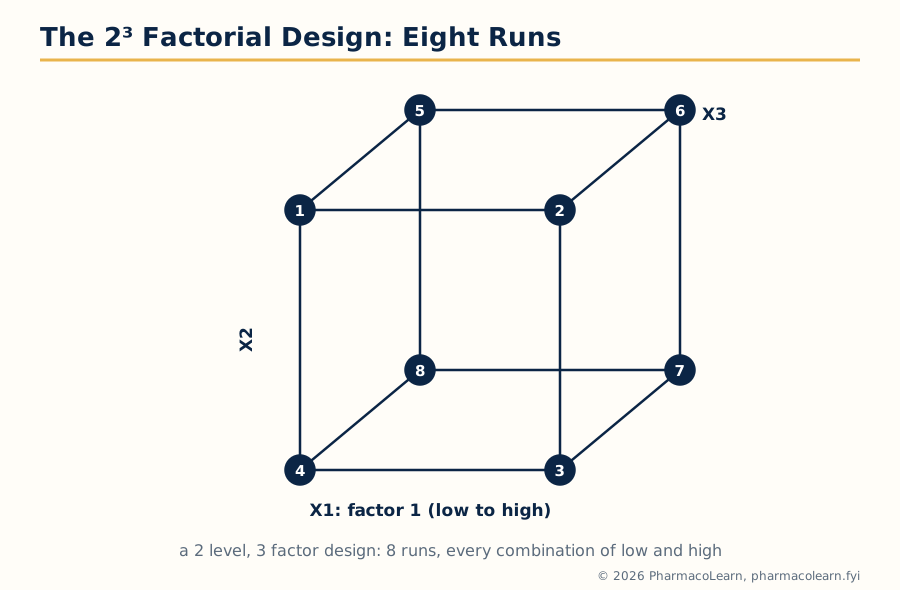 Figure: The 2 to the power 3 factorial design. Eight runs at the cube's corners measure every main effect and every interaction, which no one factor at a time programme can do.
The factorial design is the workhorse of optimization: every combination of the chosen levels of the factors is run, so each factor's effect is measured at every setting of the others. For k factors at two levels the design has 2 to the power k runs: 4 runs for two factors, 8 for three, 16 for four, small numbers that already contain far more information than the same runs spent one factor at a time. The analysis fits a polynomial model to the responses,
Y = b0 + b1 X1 + b2 X2 + b12 X1 X2 + ...
in which the coefficients b1 and b2 are the main effects of the two factors and b12 is their interaction, the term one factor at a time work can never estimate. Effects are judged against experimental error, from replicate runs or centre points (runs at the middle settings, which also test for curvature), using analysis of variance. A compact example: a tablet study with binder level (X1) and compression force (X2) at two levels each, four batches, measuring dissolution at 30 minutes, finds binder lowers dissolution, force lowers it slightly, and the interaction term shows the binder penalty grows at high force, so the optimum direction is low binder with moderate force, a conclusion no sequential tinkering would have stated so cleanly. When curvature matters, the two level design is extended with centre and axial points into response surface designs (section 3.5). When factors are numerous, full factorials grow too large and the fractional and screening designs of the next section take over.
3.4 Screening designs
Screening is the stage before optimization proper: many candidate variables, little knowledge, and the need to find the vital few that actually move the responses, so that a factorial or response surface design can be afforded on them. Screening designs run far fewer experiments than a full factorial by accepting that some effects will be entangled with each other. The fractional factorial design runs a carefully chosen fraction (a half, a quarter) of the full combinations, keeping main effects clear while confounding interactions with each other, an acceptable bargain when interactions among many factors are mostly small. The Plackett-Burman design goes further, screening up to N minus 1 factors in N runs (11 factors in 12 runs, a classic layout), estimating main effects only, on the sparsity principle that in most systems a few factors dominate. Analysis ranks the effects, by size on a normal probability plot or against a significance yardstick, and the survivors pass to the optimization designs. Screening is also the risk assessment engine of QbD (section 1.10): it converts the long list of "could matter" variables into a short, evidence based list of critical ones, and its output decides where the development budget goes.
| Design | Runs for the question | What it estimates | Stage used |
|---|---|---|---|
| Plackett-Burman | N runs for up to N minus 1 factors | Main effects only | Screening many factors |
| Fractional factorial | A half or quarter of 2^k runs | Main effects, some interactions confounded | Screening with some interaction cover |
| Full factorial, 2^k | 2^k runs | All main effects and interactions | Optimization of few factors |
| Central composite | 2^k plus centre and axial points | Full quadratic model, curvature | Response surface optimization |
| Box-Behnken | Three level combinations, no corner runs | Full quadratic model | Response surface where corners are impractical |
3.5 Optimization technology: response surfaces and the search for the optimum
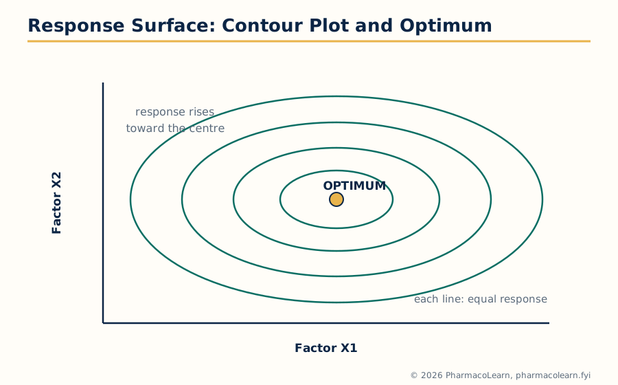 Figure: A contour plot of a fitted response surface. The formulator reads the terrain directly: where the contours crowd the response is sensitive, and the optimum sits where they close.
Optimization technology is the layer that turns fitted models into decisions. For quantitative factors and a continuous response, the fitted polynomial of section 3.3 is drawn as a response surface, or its two dimensional shadow, the contour plot, on which lines of equal response let the formulator see the ridge, valley or summit structure of the system directly. With several responses, the contour plots are overlaid and the acceptable windows intersected (the overlay plot), and the overlapping region is the formulation sweet spot, the same object as a QbD design space drawn for two variables. A formal alternative is the desirability approach: each response is converted to a desirability score between 0 (unacceptable) and 1 (at target), the scores are combined into one overall desirability, and the software searches the factor space for the settings maximising it, handling maximise, minimise and in window targets together. The search itself, over the model rather than the bench, is where the computer earns its title in this subject: grid searches and numerical optimisers evaluate thousands of candidate settings in seconds. Standard statistical and DOE software packages (the widely used examples include Design-Expert and Minitab) automate design generation, model fitting, diagnostics and this search. Two disciplines protect the result: the model must pass its checks (residual patterns, lack of fit, agreement between fitted and predicted values) before it is believed, and the predicted optimum must be confirmed by real batches, whose results are compared with the prediction as the final validation of the whole exercise.
3.6 Computers in pharmaceutical formulation: emulsions
An emulsion, oil droplets dispersed in water or the reverse, is a formulation whose quality lives in its globule size distribution and its resistance to creaming, coalescence and phase inversion, and computer methods help at each design decision. The first decision, which emulsifier and how much, is guided by the hydrophilic lipophilic balance (HLB) system, in which the required HLB of the oil phase is matched against tabulated emulsifier values and blends are calculated arithmetically, a computation software handles exactly, including the blend proportions for a target HLB. Phase behaviour studies, which map where a given oil, water and emulsifier composition forms a stable emulsion, a separated system or a gel, produce diagrams that are plotted and stored computationally, building a formulation knowledge base for the oil in question. Processing variables (homogeniser speed, time, temperature, order of addition) are optimized by the designs of this unit, with globule size and stability indices as responses. Prediction enters through stability modelling: accelerated stability data are extrapolated by statistical models to estimate shelf life, and expert system and neural network approaches reported in the literature learn from banks of past formulations to suggest starting compositions for new oils and drugs.
3.7 Microemulsion drug carriers
Microemulsions are the refined relatives of emulsions: thermodynamically stable, transparent, isotropic mixtures of oil, water and surfactant (usually with a cosurfactant) that form spontaneously with droplets in the tens of nanometres range, and that solubilise poorly soluble drugs in their oil cores and interfacial films, which is why the syllabus names them as drug carriers. Their formulation is a mapping exercise perfectly suited to the computer. The formulator titrates mixtures across the composition triangle and records where the system is a clear microemulsion, where it is turbid or separated, and software plots the results as a pseudoternary phase diagram, three components at the corners (oil, water, and surfactant with cosurfactant combined as one corner), the diagram's clear region being the territory in which carrier formulations can be chosen. Within that region, drug loading, dilution behaviour (the carrier must survive dilution in gut fluids without precipitating its drug), globule size and release are then optimized by factorial methods. Self microemulsifying drug delivery systems (SMEDDS) are the practical dosage form of the idea: an anhydrous preconcentrate in a capsule that forms a microemulsion on contact with gastrointestinal fluid, a marketed strategy for lipophilic drugs with dissolution limited absorption, and a direct bridge between this unit's phase diagrams and Unit 2's absorption modeling.
3.8 Legal protection of innovative uses of computers in R&D
Computer based innovation is valuable, so the law of its protection is part of the subject. The available instruments differ by what they protect. Patents protect inventions: a novel process, formulation or use discovered with a computer is patentable like any other, and computer implemented inventions occupy a middle ground that varies by jurisdiction, pure software and mathematical methods as such being excluded in several systems (in India, section 3(k) of the Patents Act excludes computer programmes per se, while inventions with a technical application beyond the programme itself are examined under the computer related inventions guidelines), so drafting focuses on the technical contribution, a better controlled process or a new formulation found, rather than on the code. Copyright protects the expression of software, its code and documentation, automatically on creation, but not the underlying method. Trade secrets protect confidential know how, which in this field includes trained model parameters, curated databases and the negative results of screening campaigns, for exactly as long as secrecy is maintained, and access controls and contracts are the practical protection. Databases attract their own rights in some jurisdictions, and the licensing terms of commercial software and data (what the licence permits, especially model training and redistribution of outputs) are a working legal constraint on every modelling team. The examination point is the matching: choose the instrument that fits the asset, patent the invention, copyright the code, keep the data secret, and read the licence before the model, not after the dispute.
3.9 The ethics of computing in pharmaceutical research
Computing power creates ethical exposures that this syllabus head names directly. Data integrity is the first: a computer can alter, select or regenerate data invisibly, so the ethical rule is that electronic records must be complete, attributable and preserved in original form (the regulatory machinery for this is Unit 4, section 4.11), and the temptation a spreadsheet offers, to delete the awkward point, is exactly the falsification that ends careers and licences. Honest modelling is the second: a simulation reported without its assumptions, or a model tuned until it agrees with the desired answer, misleads patients and regulators as surely as fabricated data; the ethics are the statistics of Unit 1 read as duties, report the confidence region, the sensitivity, the failed checks. Credit and authorship is the third: work done by shared software, databases and, now, generative artificial intelligence must be attributed accurately, and submitting machine generated text or analysis as one's own unaided work breaches the same honesty rule in examinations and publications alike. Animal and human welfare is the fourth, and it cuts the other way: good in silico work is an ethical good, because prediction that replaces an animal study or a doomed clinical trial follows the replacement principle of the 3Rs, while careless prediction that sends a bad molecule into animals or patients is an ethical failure, not merely a technical one. Finally, bias and access: models trained on unrepresentative data inherit its blind spots, a point that returns with artificial intelligence in Unit 5.
3.10 Computers in market analysis
The last head of this unit leaves the laboratory for the business the laboratory serves. Pharmaceutical market analysis is data work: companies buy and analyse prescribing and sales audit data (the large commercial audits of which IQVIA is the best known supplier), hospital and retail panel data, and epidemiological estimates of disease prevalence, and model them to answer development questions. Which indication and patient population justify a programme. How large is the treated population, and how will diagnosis and treatment rates change. What will a new product's uptake curve look like against entrenched competitors, modelled from analogue launches and the product's modelled profile. When will patent expiry expose the brand to generics, and what is the product worth across its lifecycle under price and competition scenarios. The techniques are those of Unit 1 in commercial dress: regression and time series forecasting, sensitivity analysis over price and uptake assumptions, and scenario simulation. The connection to the rest of the subject is direct: the target product profile that opens a QbD programme (section 1.10) is written from market and clinical analysis of exactly this kind.
The optimization workflow of Unit 3
Define responses and targets
   |
   v
Choose variables and ranges
   |
   v
Screening design: find the vital few factors
   |
   v
Factorial or response surface design: fit the model
   |
   v
Check the model: residuals, lack of fit
   |
   v
Predict the optimum on the model, confirm at the bench
Unit 4: Computer Aided Biopharmaceutical Characterization, PK/PD Simulation and Clinical Development
4.1 Gastrointestinal absorption simulation: introduction and theoretical background
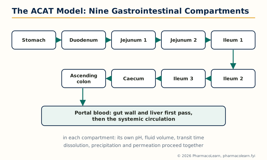 Figure: The ACAT model of gastrointestinal absorption simulation. The dose transits nine compartments, each with its own pH, fluid volume and transit time, dissolving and permeating as it goes.
Gastrointestinal absorption simulation predicts the plasma profile of an oral dose before the dose is ever given to a human, by simulating the journey MPH202T described: disintegration, dissolution, transit through changing gut conditions, permeation, gut wall and liver first pass, and entry into a pharmacokinetic model of the body. The theoretical core is the compartmental absorption and transit (CAT) model and its advanced form, the ACAT model, which divides the gastrointestinal tract into nine compartments: stomach, duodenum, two jejunal and three ileal segments, caecum and ascending colon. Each compartment carries its own pH, fluid volume, surface area and transit time, and the dose moves through them in sequence, dissolving, possibly precipitating, permeating and being degraded at compartment specific rates, while absorbed drug passes the gut wall (with its transporters and enzymes, Unit 2) and the liver before reaching the systemic model. The governing mathematics is a chain of mass balance differential equations, one set per compartment, integrated numerically. The commercial platforms built on this theory, GastroPlus being the widely used example, and the PBPK platforms such as the Simcyp simulator for the systemic side, are the working instruments of the sections that follow. The value of the exercise is foresight: formulation variants, doses, food effects and special populations can be compared in silico, and the expensive experiments reserved for the questions the model cannot settle.
4.2 Model construction
Building an absorption simulation follows a fixed discipline. First, assemble the compound inputs: molecular weight, pKa values, log P and its pH dependence, solubility as a function of pH (section 2.4), permeability (section 2.5), plasma protein binding, blood to plasma ratio, and clearance mechanisms, each flagged by source, measured, predicted in silico or taken from the literature, because the output can be no better than the weakest input. Second, add the formulation inputs: dose, dosage form type, particle size distribution, and the measured dissolution profile, which the model converts into in vivo release. Third, choose the physiology: the standard fasted or fed gut model, or a population variant for age, disease or species. Fourth, run and compare: simulated against any observed data that exist, from animal studies or earlier clinical work, with the model accepted for prediction only where it reproduces what is known, the verification step that separates simulation from speculation. Fifth, document the assumptions: software models used for decisions, and especially for regulatory submissions, carry a record of inputs, versions and checks.
4.3 Parameter sensitivity analysis in absorption simulation
Unit 1 defined sensitivity analysis generally; in absorption simulation it has a specific job, because the input list of section 4.2 mixes well measured numbers with rough predictions, and the user must know which uncertainty matters. The platform varies one input at a time (solubility across its plausible range, permeability likewise, particle size, gastric emptying time) and reports the effect on the outputs that drive decisions: fraction absorbed, Cmax and AUC. The standard lessons recur. For a BCS class II drug the output is exquisitely sensitive to solubility and particle size and almost indifferent to permeability, so the formulation budget goes to dissolution. For a class III drug the pattern reverses. A prediction robust across the plausible range of every uncertain input can be carried forward with confidence; a prediction that flips when one poorly known input moves is a finding in itself, it identifies the single experiment most worth doing. Parameter sensitivity analysis is thus the bridge between the virtual work of this unit and the bench work it directs.
4.4 The virtual trial
A virtual trial runs the simulation not for one standard subject but for a population of virtual subjects, each assembled by sampling physiology and drug parameters from their distributions: gastric pH and emptying, transit times, enzyme and transporter abundance, body size, plasma binding, and the variability of the compound inputs themselves. The machinery is Monte Carlo simulation, hundreds or thousands of runs whose results are summarised as a distribution of outcomes, a mean profile with its spread, the fraction of subjects outside a target window, the predicted variability a real trial should expect. Virtual trials answer questions no single run can: whether a formulation robust in the average subject stays robust in slow emptiers; what sample size a bioequivalence study needs given predicted variability; how a dose performs across renal function or age bands before those patients are exposed. They are the population modeling of section 1.9 turned forward, from analysing data to generating it, and they inherit its ethics (section 3.9): a virtual trial that replaces an uninformative real trial is a gain, while one that overstates its certainty to skip a necessary trial is a hazard.
4.5 Fed versus fasted state simulation
Food changes oral absorption through several mechanisms at once: gastric pH rises, emptying slows, bile salt and lipid concentrations in the intestine climb (raising the solubility of lipophilic drugs), splanchnic blood flow increases, and the dosage form itself may behave differently, including the risk of dose dumping from some modified release products. Clinical food effect studies are therefore standard, and predicting them is a prized simulation task. The fed state model adjusts the physiology compartment by compartment: longer gastric residence, higher intestinal solubilisation capacity through bile micelles, altered fluid volumes and transit, and the compound's measured solubility in fed state simulated media feeds the dissolution side. A model that reproduces the observed fasted profile and then, with only the physiology switched, predicts the fed profile and its direction, exposure up, down or unchanged, has demonstrated the mechanistic credibility of section 1.3. Such predictions guide whether the product is labelled with or without food, whether a food effect study can be argued unnecessary, and which formulation changes would blunt an unwanted food effect.
4.6 In vitro dissolution and in vitro in vivo correlation in simulation
Within a simulation platform, a validated Level A relationship turns formulation questions into computations: change the coating, predict the new dissolution, and read off the predicted plasma consequence, which is the computational heart of biopharmaceutical characterization and the technical basis of the biowaiver argument next.
| IVIVC level | What is correlated | Predictive power |
|---|---|---|
| Level A | Whole dissolution curve against whole in vivo absorption curve, point to point | Predicts the plasma profile; dissolution can serve as a surrogate |
| Level B | Mean in vitro dissolution time against mean in vivo residence or absorption time | Summary only; several profiles share one mean, so profiles cannot be predicted |
| Level C | One dissolution measurement against one PK parameter (Cmax or AUC) | Screening and quality use; no profile prediction |
4.7 Biowaiver considerations
A biowaiver is a regulatory decision to approve a product, or a change to one, without a new in vivo bioequivalence study, on the strength of in vitro and in silico evidence. The established BCS based biowaiver (MPH202T, section 4.8) waives the study for rapidly dissolving immediate release products of high solubility drugs under defined conditions, because gastric emptying, not formulation, controls their absorption. Simulation extends the reasoning: a verified absorption model, exercised across the plausible range of product and patient variation (the virtual trial of section 4.4), can argue that two formulations cannot differ in vivo by more than a stated amount, or that a manufacturing change or site transfer leaves exposure unchanged. The regulatory posture is deliberately cautious, and the considerations that decide acceptance are consistent: the model must be verified against observed data for the same or closely related products; its sensitive parameters (section 4.3) must be measured, not guessed; the claim must stay inside the conditions the evidence covers; and the consequence of error must be proportionate, a biowaiver argument for a narrow therapeutic index drug faces a far higher bar. Simulation supports biowaivers; it does not yet replace the judgement that grants them.
4.8 Computer simulations in pharmacokinetics and pharmacodynamics: the whole organism
At the whole organism level, PK simulation means the compartmental and PBPK models of Unit 2 run forward in time: dose in, predicted concentration time curve out, for any regimen, route or population the model is built to represent. Its routine uses are regimen design (loading and maintenance doses from clearance and volume), prediction of accumulation and time to steady state (MPH202T, Unit 3), interaction prediction (an inhibitor's effect entered as a change in the relevant clearance and the new steady state computed), and trial design, where simulations fix sampling schedules (with optimal design, section 1.8) and expected variability before patients are recruited. Pharmacodynamic simulation joins an effect model, most often the saturable Emax relationship of MPH202T section 5.3, possibly with delays for distribution to the effect site or indirect mechanisms such as cell turnover, so that the output is effect against time: onset, peak, duration, and the consequence of missed or doubled doses. Population platforms combine both with the variability machinery of section 1.9, so a development team can ask, and answer numerically, what fraction of the target population a proposed dose puts inside the therapeutic window.
4.9 Simulation at the levels of tissues, organs, cells, proteins and genes
The syllabus descends the biological scale, and each level has its simulation style. Isolated tissues and organs: perfused organ and tissue bath preparations are modeled as small systems in their own right, concentration in the bath, uptake into the tissue, response as a function of exposure, and such models both interpret preclinical experiments and feed parameters upward into PBPK tissue compartments. Cells: cell level models describe transport across the cell membrane, intracellular binding and metabolism, and the signalling cascades by which a receptor event becomes a cellular response, systems of differential equations for pathway components, the quantitative core of systems pharmacology. Proteins: at the molecular level, docking predicts how a ligand sits in a binding site, and molecular dynamics simulates the protein and ligand moving in solvent over time, estimating binding stability and the conformational changes behind agonism and resistance mutations. Genes: gene level work is computational genomics and network modeling, expression data analysed for pathway activity, genetic variants in enzymes and transporters (Unit 2) entered as parameter changes in the higher level models, so that a polymorphism in a clearance enzyme becomes, computationally, a different virtual patient.
4.10 Computers in clinical development: clinical data collection and management
Clinical trials are the most expensive data pharmaceutical science collects, and computers run their collection. The paper case report form has given way to electronic data capture (EDC): investigators enter data on electronic case report forms with built in range and consistency checks at the point of entry, patients increasingly report outcomes directly through electronic patient reported outcome devices and diaries, and laboratory and imaging data flow in electronically from central facilities. Behind the forms sits the clinical data management system and its discipline: a data management plan, edit checks programmed against the protocol, queries raised and resolved with sites, coding of adverse events and medications against standard dictionaries (MedDRA for events, the WHO drug dictionary for medicines), reconciliation against safety databases, and finally database lock, the frozen, auditable state from which statisticians analyse. International data standards (the CDISC family, including the SDTM structure for tabulated study data) make trial datasets machine readable and submittable in a form regulators can analyse directly.
4.11 Regulation of computer systems
Because regulated decisions rest on electronic records, the systems holding them are themselves regulated. The landmark instrument is the US FDA's 21 CFR Part 11 (1997), which sets the conditions under which electronic records and electronic signatures are considered trustworthy equivalents of paper and ink: system validation, secure audit trails that record who created, changed or deleted a record and when, authority checks limiting users to their roles, record retention and accurate copies for inspection. The European counterpart is Annex 11 to the EU GMP guide, and the industry's working framework for achieving compliance is the GAMP guide (Good Automated Manufacturing Practice, published by ISPE), which classifies software by category and scales the validation effort to risk. Underneath the rules sits one principle, data integrity, summarised in the ALCOA expectations: records must be attributable, legible, contemporaneous, original and accurate. Validation is the documented demonstration that a system does what it is intended to do, from specification through testing to controlled change, and it applies to the instruments of this whole subject, the LIMS, the EDC platform, the manufacturing automation and the modelling software used in submissions, where the credibility of a simulation is partly the credibility of the validated system that produced it.
The gastrointestinal absorption simulation workflow
Compound inputs: solubility, pKa, log P, permeability
   |
   v
Formulation inputs: dose, particle size, dissolution profile
   |
   v
ACAT model: nine gut compartments, transit and pH
   |
   v
Gut wall and liver first pass (transporters, Unit 2)
   |
   v
Systemic PK model: plasma profile out
   |
   v
Verify against observed data, then predict:
fed state, new formulations, virtual populations
Unit 5: Artificial Intelligence, Robotics and Computational Fluid Dynamics
5.1 Artificial intelligence: a general overview
Artificial intelligence (AI) is the branch of computer science concerned with systems that perform tasks which, done by a human, would be called intelligent: recognising patterns, learning from examples, and making predictions or decisions. Its working core in current practice is machine learning, in which the system's rules are not written by a programmer but estimated from data: given many examples of inputs with their known outputs, an algorithm adjusts its internal parameters (the estimation of Unit 1, at industrial scale) until its predictions on new inputs are accurate. The main styles are supervised learning, trained on labelled examples (this structure, that measured solubility); unsupervised learning, which finds structure such as clusters in unlabelled data; and reinforcement learning, which improves by trial and reward. Deep learning, the family behind most recent advances, uses neural networks of many layers that learn their own internal features from raw inputs such as molecular graphs, images and text, at the cost of large data requirements and decisions that are hard to inspect, the black box problem. Two disciplines from Unit 1 govern whether an AI result is worth anything: the model must be validated on data it never saw in training, and a model with too much freedom will memorise its training set and fail on new cases, the overfitting of section 1.4. AI is best understood as this subject's statistical modelling grown powerful and data hungry, not as an exemption from it.
5.2 Artificial intelligence in pharmaceutical research and development
AI applications now appear at every stage this subject has visited. In discovery, models predict activity, solubility, permeability and toxicity from structure (the QSAR of section 1.1 grown into deep learning), screen virtual libraries of millions of compounds, and generate entirely new candidate structures optimised against several properties at once; protein structure prediction by systems such as AlphaFold has given modelers targets that were previously unmodelled. In preclinical and clinical development, AI reads images and signals (pathology slides, ECGs, retinal scans), predicts which patients match a trial's biology, forecasts recruitment and flags data anomalies in the clinical databases of section 4.10. In formulation and manufacturing, learning models predict formulation behaviour from composition and process data, detect defects and drift from sensor and image streams beyond human vigilance, and support the control strategies of section 1.10. The working cautions are equally standard: an AI model is only as good as its training data, which in pharmacy are often small, biased toward successes and expensive to generate; performance on familiar chemistry does not guarantee performance on new chemistry; and for regulated uses the model must be validated, versioned and explainable enough for a reviewer to judge, requirements the field is still formalising.
5.3 Robotics and pharmaceutical automation
A robot is a programmable machine that senses, decides and physically acts: it moves materials, manipulates laboratory ware and executes procedures. Pharmaceutical automation is the wider term the syllabus pairs with it, covering robots proper, automated instruments, conveyor and storage systems, and the software that schedules and records them, wherever physical or routine work is mechanised under computer control. In the laboratory, liquid handling robots prepare plates and dilutions, automated systems run high throughput screening and stability storage, and robotic arms tend instruments around the clock. In manufacturing, automation fills, inspects, packs and labels at speeds and consistency beyond manual work, moves materials in warehouses and cleanrooms, and operates the process equipment whose sensors feed the PAT and control systems of Unit 1. In the pharmacy itself, automated dispensing and compounding systems prepare individualised doses, including hazardous cytotoxic preparations, with barcode checked accuracy.
5.4 Pharmaceutical applications of AI, robotics and CFD
Read across the three technologies of this unit, the application map is complementary: AI decides and predicts, robotics and automation act and execute, and computational fluid dynamics (sections 5.6 and 5.7) simulates the physical processes the other two must control. A modern development programme uses all three together: AI proposes the formulation and predicts its behaviour, CFD checks that the granulator or coater will treat every particle alike at scale, automation runs the process identically every time, and the data from every run train the next round of models. Concrete applications include automated high throughput formulation screening in which robots prepare hundreds of prototype variants for AI ranked evaluation, and continuous manufacturing lines whose flow fields are CFD designed and whose quality is held by automated, model based control.
| Technology | Core strength | Representative pharmaceutical applications |
|---|---|---|
| Artificial intelligence | Learning patterns and predictions from data | Property and toxicity prediction, virtual screening, image based QC, formulation prediction |
| Robotics and automation | Physical execution with speed and reproducibility | High throughput screening, liquid handling, automated filling and inspection, dispensing |
| Computational fluid dynamics | Simulating flow, mixing and transfer in equipment | Mixer and granulator design, fluid bed coating, cleanroom airflow, inhaler aerosol flow |
5.5 Advantages and disadvantages of AI, robotics and automation
The advantages recur across applications. Speed and throughput rise by orders of magnitude in screening, data handling and physical processing. Reproducibility improves because machines execute the written procedure identically and record it completely, strengthening both quality and the data integrity of section 4.11. Hazardous and tedious work, cytotoxic compounding, repetitive weighing, round the clock monitoring, moves from people to machines. Prediction shortens development: programmes fail earlier and cheaper, in silico rather than in patients. The disadvantages are the mirror images. Capital and validation costs are high, and a validated automated system is expensive to change, which can freeze a process the science wants to improve. AI inherits the limits of its data and can fail silently outside them, while its opacity complicates the explainability regulators require. Automation deskills some roles and demands new ones, programmers, data scientists, validation specialists, that are scarce. And dependence is itself a risk: when the system is down or wrong, an organisation that has lost the manual skill has lost its fallback. The balanced syllabus position, and the industrial one, is selective adoption: automate the routine, predict the predictable, and keep human judgement on the exceptions and the accountability.
5.6 Computational fluid dynamics: a general overview
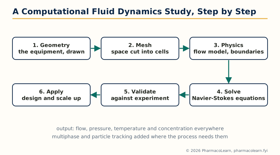 Figure: The anatomy of a CFD study. The validation step is not optional: an unvalidated simulation is a coloured picture, not evidence.
Computational fluid dynamics (CFD) simulates the movement of fluids, and with them heat, dissolved drug and suspended particles, by solving the equations of fluid motion numerically. The governing equations are the Navier-Stokes equations, the conservation laws for mass, momentum and energy applied to a moving fluid, which have no general pencil and paper solution for real geometries. CFD replaces the continuous space with a mesh of many small cells, writes the conservation equations for each cell, and solves the enormous resulting system iteratively on the computer until flows, pressures, temperatures and concentrations are known everywhere in the equipment. A CFD study has a standard anatomy: define the geometry (a stirred tank, a fluid bed coater, a dry powder inhaler), generate and check the mesh, set the physics (single or multiphase flow, a turbulence model where the flow demands one, particle tracking for suspended solids), set boundary and operating conditions, solve, and validate against experiment, because an unvalidated CFD model is a coloured picture, not evidence.
5.7 CFD in pharmaceutical applications
The established applications follow the unit operations of pharmaceutics. In mixing, CFD predicts blend uniformity and mixing time in stirred tanks and blenders, locates dead zones, and supports scale up by holding the right quantity constant, tip speed, power per volume or shear, a choice the simulation can test rather than assume. In granulation and coating, fluidised bed processes are simulated with gas flow coupled to particle motion, predicting coating uniformity, drying rates and the conditions that cause agglomeration or attrition, directly serving the products of MPH201T and MPH203T's own formulation work. In drying and lyophilisation support operations, airflow and heat transfer models size and arrange equipment evenly. In cleanrooms and sterile manufacture, CFD verifies that air change patterns sweep contaminants away from critical zones as designed. In inhalation products, aerosol flow through inhaler devices and the human airways is simulated to predict where particles deposit, linking device design to the pulmonary delivery of MPH201T. Across all of these the workflow is the same as Unit 4's, geometry and physics in, verified prediction out, and the answer used to run fewer, better experiments.
5.8 Current challenges
The challenges facing the technologies of this subject are shared and specific. Data are the first: models of every kind in this subject are limited by the quantity, quality and representativeness of pharmaceutical data, much of which is proprietary, negative, unrecorded or locked in incompatible systems. Validation and regulatory acceptance form the second: a prediction used in a submission must carry its evidence of correctness, and frameworks for crediting models, especially learning models that change as they are retrained, are still maturing on both sides of the submission table. The third is integration: discovery, development, manufacturing and clinical systems were bought at different times from different vendors, and the informatics vision of the subject, one coherent flow of data from molecule to patient, is still more aspiration than fact in most organisations. The fourth is people: the field needs scientists fluent in both pharmaceutics and computation, and they remain rarer than either skill alone.
5.9 Future directions
The direction of travel is toward integration and autonomy. Digital twins, living simulation models of a process or a product, updated continuously with its real data, are the stated goal of both manufacturers and regulators: a twin of a continuous line that predicts quality minutes ahead and adjusts the process, and in time a twin of a patient population in which doses are tested before they are prescribed. Model informed drug development is becoming the default regulatory language, with simulation evidence expected, not merely accepted, in areas from paediatric extrapolation to interaction labelling. Continuous manufacturing binds this unit's three technologies into one line: CFD designed equipment, automation executing, AI supervising. And AI itself is becoming generative, proposing molecules and experiments rather than only scoring them, which raises the premium on this subject's oldest lessons: every model, however modern, stands or falls on the estimation, validation and honest uncertainty of Unit 1.
The subject in one chain
Statistics and QbD frame every model (Unit 1)
   |
   v
Disposition is predicted, transporters included (Unit 2)
   |
   v
Formulations are optimized by designed experiments (Unit 3)
   |
   v
The gut, the trial and the clinic are simulated (Unit 4)
   |
   v
AI, robots and CFD extend the same logic (Unit 5)
Frequently Asked Questions
Q: What is the difference between a descriptive and a mechanistic model? A descriptive model reproduces the pattern in the data with an equation whose parameters need have no physical meaning, such as a polynomial fitted to a dissolution profile; it interpolates well but cannot be trusted outside the studied range. A mechanistic model is built from the processes believed to generate the data, dissolution, permeation, transit, clearance, so its parameters are physical quantities and it can extrapolate to new doses, formulations and populations, at the price of needing more knowledge and more data.
Q: What is population modeling, and why is it used in drug development? Population modeling fits data from all subjects at once, separating fixed effects (typical parameter values and the influence of covariates such as weight, age and renal function) from random effects (variability between and within subjects). It works on the sparse, unbalanced samples real trials produce, describes the whole distribution of behaviour rather than an average patient, and supports dose decisions for special populations who differ from the average.
Q: What does ICH Q8 require, and what is a design space? ICH Q8 is the guideline on pharmaceutical development that defines Quality by Design: development beginning from a quality target product profile, identifying critical quality attributes, assessing risk, and building process understanding through designed experiments and models. The design space is the multidimensional region of material attributes and process parameters demonstrated to assure quality; working inside it is not treated as a regulatory change, while moving outside it is.
Q: Why must transporters such as P-gp be modeled explicitly in drug disposition? Because they break the passive diffusion picture. Efflux transporters such as P-gp and BCRP pump substrates back into the gut lumen, into bile or out of the brain, and uptake transporters such as OATP and hPEPT1 decide whether other drugs enter the body or the liver at all. A substrate's absorption, distribution and interactions cannot be predicted from solubility and lipophilicity alone; the transporter step has to be in the model, saturable and inhibitable, as Unit 2 sets out.
Q: How is a factorial design better than changing one factor at a time? A factorial design runs every combination of factor levels, so each factor's effect is measured at all settings of the others and the interactions between factors become estimable, which one factor at a time experiments can never detect. It also extracts more information from the same number of runs, and its fitted polynomial model predicts the response across the whole studied region, not only along the path the experimenter happened to walk.
Q: What is a screening design, and when is it used? A screening design identifies the few influential factors among many candidates using very few runs, by estimating main effects while accepting that interactions are confounded, as in Plackett-Burman designs that screen up to eleven factors in twelve runs. It is used at the start of development, and inside QbD risk assessment, to decide which variables deserve the full factorial or response surface study that follows.
Q: What is a virtual trial? A virtual trial is a simulation run over a population of virtual subjects, each sampled from distributions of physiology and drug parameters, instead of a single standard subject. Its output is a distribution of outcomes: mean profiles with spread, the fraction of subjects inside a target window, the variability a real trial should expect. Virtual trials size real studies, test robustness across populations and can replace trials that would be uninformative, provided their uncertainty is honestly reported.
Q: How can gastrointestinal absorption simulation support a biowaiver? A biowaiver waives an in vivo bioequivalence study on in vitro evidence. A verified absorption simulation strengthens the argument by exercising the model across the plausible range of formulation and patient variation, virtual trial style, and showing that the compared products cannot differ in exposure beyond a stated amount. Acceptance requires the model to be verified against observed data, its sensitive parameters to be measured rather than guessed, and the claim to stay within the conditions the evidence covers.
Q: What does 21 CFR Part 11 require of a computer system used in clinical development? Part 11 sets the conditions for electronic records and signatures to be trusted as equivalents of paper records: the system must be validated, keep secure audit trails recording who created, changed or deleted each record and when, restrict users by authority checks, and retain records in accurate, inspectable form. The European counterpart is GMP Annex 11, and both rest on data integrity: records that are attributable, legible, contemporaneous, original and accurate.
Q: What is the difference between artificial intelligence, robotics and automation in pharmacy? Artificial intelligence is software that learns from data and makes predictions or decisions, such as forecasting a molecule's solubility or reading a quality control image. Robotics is machinery that physically acts in the world, handling plates, filling vials or compounding doses. Pharmaceutical automation is the wider system joining robots, instruments and control software so that a whole routine process runs, records itself and stays in control with minimal manual intervention.
Complete MPH203T notes, all 5 units in one PDF, free to keep.
Other M.Pharm subjects: MPH101T · MPC101T · MPL101T · MPH102T · MPH103T · MPH104T · MPL102T · MPL103T · MPL104T · MPC102T · MPC103T · MPC104T · MPH201T · MPH202T · MPH203T · MPH204T · MPC201T · MPC202T · MPC203T · MPC204T · M.Pharm