
MPH103T — Modern Pharmaceutics
4 hrs/week, 4 credits, 60 hours, 100 marks. Notes follow the M.Pharm syllabus, unit by unit.
MPH103T Modern Pharmaceutics notes for M.Pharm Semester 1 Pharmaceutics: preformulation, stability kinetics, dispersions, parenterals, optimization, validation, cGMP, tablet compression, Heckel plots and statistics, with free unit wise PDF downloads on PharmacoLearn.
Units in this subject
- Unit 1 — Preformulation Concepts, Pharmaceutical Dispersions, Parenterals and Optimization Techniques
- Unit 2 — Validation
- Unit 3 — cGMP and Industrial Management
- Unit 4 — Compression and Compaction
- Unit 5 — Consolidation Parameters, Dissolution Models and Pharmaceutical Statistics
Download MPH103T PDF Notes
Free PDFs for this subject, one per unit:
Modern Pharmaceutics, subject code MPH103T, is a core Semester 1 subject of M.Pharm Pharmaceutics. It carries 4 credits and 60 hours of theory, taught at 4 hours per week, for 100 marks.
This subject is about how a pharmaceutical product is developed and manufactured in industry. Before a formulation is made, the drug and its excipients are characterised in preformulation studies and checked for compatibility and stability. The formulation is then improved systematically by optimization techniques and statistical designs instead of trial and error. In the factory, validation proves that facilities, equipment and processes do what they are supposed to do, and current good manufacturing practice (cGMP) with sound industrial management keeps production under control. The last two units deal with the physics of tablet compression, where a powder is consolidated into a compact, and with the parameters and statistics used to judge consolidation, dissolution and drug release profiles. A student who completes this subject should be able to design preformulation studies, interpret stability and dissolution data with the standard models and tests, and explain how an industrial process is qualified and kept in a validated state.
Unit 1: Preformulation Concepts, Pharmaceutical Dispersions, Parenterals and Optimization Techniques
1.1 Preformulation studies: scope and parameters
Preformulation is the stage of development in which the physicochemical properties of a new drug substance are characterised, alone and in combination with excipients, before a dosage form is designed. It is the first step in the rational development of a dosage form. The information generated decides which dosage form is feasible, which excipients are safe to combine with the drug, what processing route to choose, and what stability problems to expect.
The main studies are:
- Organoleptic and bulk properties: colour, odour, taste, crystal form and polymorphism, particle size and size distribution, powder flow, density and hygroscopicity.
- Solubility profile: solubility in water and in solvents of different pH, pKa and ionisation behaviour, partition coefficient, dissolution behaviour of the solid.
- Stability profile: stability of the drug in solid state and in solution, the effect of pH, temperature, light and oxygen, and identification of the main degradation pathways.
- Compatibility studies: interaction of the drug with the excipients that are likely to be used, tested before the formulation is finalised (section 1.2).
- Derived properties for processing: compressibility, compactibility and flow, which decide between direct compression, granulation and other routes.
Preformulation data save time and money later. A drug that is poorly soluble will need a solubility strategy; a drug that is moisture sensitive will need protective packaging and a dry process; a drug that reacts with lactose cannot be put into a tablet that contains lactose. All of this is cheaper to learn on a few grams of drug than on a production batch.
Preformulation study sequence
Drug substance received
        |
        v
Characterisation: identity, purity, crystal form, particle size
        |
        v
Solubility and ionisation profile (pKa, log P, pH solubility)
        |
        v
Stability in solid state and solution (heat, light, pH, oxygen)
        |
        v
Excipient compatibility screening
        |
        v
Report: recommended dosage form, excipients, process and packaging
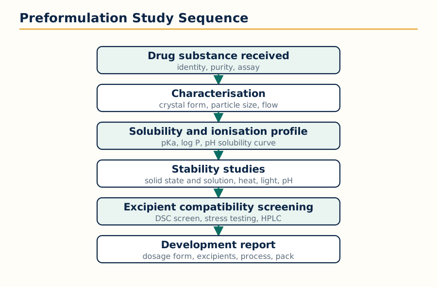 Figure: The preformulation study sequence: each stage produces information the next stage needs, ending in a development report that fixes the dosage form, excipients, process and packaging.
1.2 Drug excipient interactions: types and mechanisms
An interaction between a drug and an excipient is any change in the physical or chemical nature of the drug caused by the excipient, or a change in the excipient caused by the drug, which can alter stability, dissolution, bioavailability or appearance of the product. Some interactions are wanted (for example a solubiliser improving dissolution), but most preformulation work is about detecting unwanted ones early.
Interactions are grouped as:
- Physical interactions: no chemical reaction, but the physical state or availability of the drug changes. Examples: adsorption of a drug onto a finely divided excipient, complexation (for example tetracyclines chelating with calcium and magnesium salts), formation of eutectic mixtures that melt or soften during processing, and changes in crystal form induced by an excipient.
- Chemical interactions: a true chemical reaction that degrades the drug or forms a new entity. Common mechanisms are hydrolysis promoted by the moisture or pH microenvironment of an excipient, oxidation catalysed by trace metals or peroxide impurities in polymers, and the Maillard reaction between primary amine drugs and reducing sugars such as lactose, which causes browning and potency loss.
- Biopharmaceutical interactions: the excipient changes the release or absorption of the drug without a chemical reaction, for example a lubricant film of magnesium stearate slowing wetting and dissolution, or a surfactant changing membrane permeability.
| Interaction | Typical pair | Result if undetected |
|---|---|---|
| Maillard reaction | Primary amine drug + lactose | Browning, loss of potency |
| Chelation | Tetracycline + calcium or magnesium salts | Poor absorption of the antibiotic |
| Adsorption | Drug + colloidal silicon dioxide or clays | Slow or incomplete release |
| Hydrolysis promotion | Ester or amide drug + moist alkaline excipient | Degradation on storage |
| Oxidation catalysis | Oxidation prone drug + peroxide impurities in PEG or povidone | Degradants, discolouration |
| Eutectic formation | Two low melting solids mixed together | Softening, sticking during compression |
1.3 Methods for studying drug excipient interactions
Several methods are used together, because no single technique proves or excludes an interaction.
Thermal methods. Differential scanning calorimetry (DSC) is the most used screening tool. The drug, each excipient and the binary mixtures (often 1:1) are scanned. A shift, broadening or disappearance of the drug melting endotherm, or a new peak, suggests an interaction or a physical change such as dissolution of the drug in a molten excipient. DSC is fast and needs little sample, but a changed thermogram is only an indication: it must be confirmed by another method, because some changes are simple physical effects. Differential thermal analysis (DTA) and thermogravimetric analysis (TGA) support the same conclusions.
Spectroscopic methods. Infrared spectroscopy compares the spectrum of the drug with that of the mixture; disappearance or shifting of characteristic peaks points to interaction. UV spectroscopy, NMR and mass spectrometry are used in solution studies and for identifying degradation products.
Chromatographic methods. Thin layer chromatography and HPLC of stressed mixtures detect new spots or peaks, that is, actual degradation products. HPLC with assay and related substances measurement is the most convincing evidence because it quantifies the loss of drug.
Isothermal stress testing. Mixtures of drug and excipient, often with a small amount of added water, are stored at an elevated temperature (commonly 40 to 50 degrees Celsius) for a fixed period, then examined for physical changes (colour, liquefaction, caking) and analysed chemically. This imitates storage stress in a short time.
Other methods. X-ray powder diffraction detects changes in crystallinity; microscopy shows physical changes such as crystal growth or melting; slurry and solution studies in the presence of the excipient measure pH shifts and degradation rates. A practical programme uses DSC for rapid screening, isothermal stress testing for confirmation, and HPLC to quantify any real degradation.
1.4 Kinetics of stability
Stability kinetics describes how the rate of a degradation reaction depends on concentration, and it is the basis for predicting shelf life. The rate of reaction is the change in concentration of drug with time. For a reaction in which drug A degrades, the order of the reaction states how the rate depends on the concentration of A.
- Zero order: the rate is independent of the concentration of the reactant. Rate = k0, and concentration falls linearly with time: C = C0 minus k0 t. Suspensions often show apparent zero order behaviour because the dissolved concentration stays constant while solid remains. The half life depends on the starting concentration.
- First order: the rate is proportional to the concentration remaining. Log concentration falls linearly with time. Most drug degradation reactions are first order or pseudo first order. The half life, t1/2 = 0.693/k, is independent of the starting concentration.
- Second order: the rate depends on the concentration of two reactants, or on the square of one concentration. Less common for single drug degradation, but seen in bimolecular reactions.
Two derived times are used constantly:
- t1/2 (half life): time for the concentration to fall to half its initial value.
- t90 (shelf life): time for the concentration to fall to 90 percent of the initial value, that is, 10 percent degradation, which is the usual limit for acceptable potency. For a first order reaction, t90 = 0.105/k.
Temperature is the strongest accelerator of degradation. The Arrhenius equation relates the rate constant to temperature: k = A e raised to (minus Ea/RT), where Ea is the activation energy and A is a frequency factor. A plot of log k against 1/T is a straight line, so rate constants measured at several elevated temperatures can be extrapolated to room temperature to predict the shelf life before long term data exist. The Q10 rule is a rough shortcut from the same idea: many reaction rates roughly double or triple for each 10 degree rise in temperature. Other factors that affect the rate are pH (many drugs have a pH of maximum stability), light, oxygen, moisture, ionic strength, and the presence of catalysts such as trace metals.
Effect of temperature on degradation (Arrhenius approach)
Store samples at 40, 50, 60, 70 degrees Celsius
        |
        v
Assay at intervals, find k at each temperature
        |
        v
Plot log k against 1/T (straight line)
        |
        v
Extrapolate the line to 25 degrees Celsius to get k25
        |
        v
Shelf life t90 = 0.105 / k25 (for first order degradation)
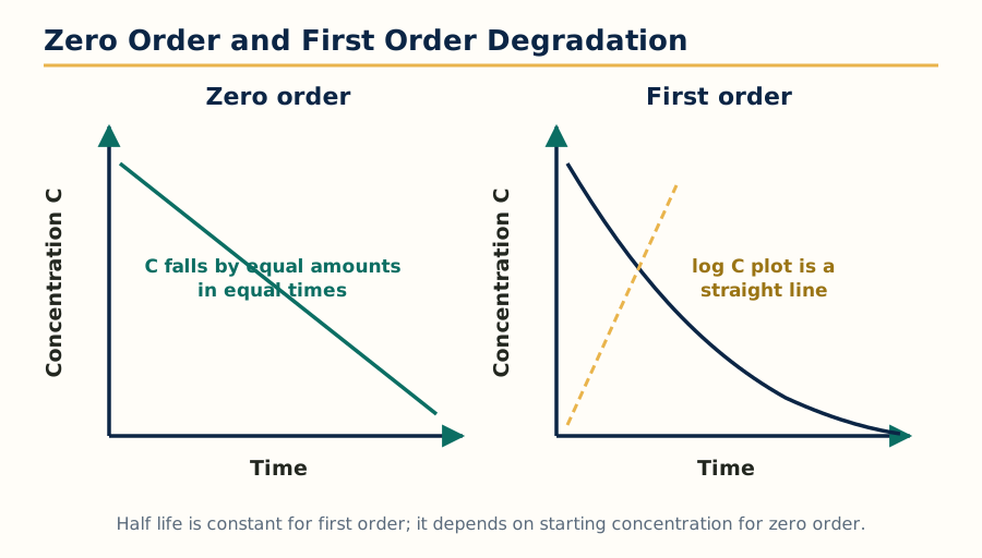 Figure: Zero order degradation loses equal amounts in equal times, while first order degradation follows an exponential curve whose log plot is a straight line.
1.5 Stability testing
Stability testing is the formal programme of studies that shows how the quality of a drug substance or product varies with time under the influence of temperature, humidity and light, and it establishes the shelf life and storage conditions printed on the label. The ICH guidelines (mainly Q1A) harmonise the design: the world is divided into climatic zones, and long term conditions are set for each zone. India falls in Zone IV, the hot and humid zone, so long term testing of products for the Indian market is commonly done at 30 degrees Celsius and 65 or 75 percent relative humidity.
A standard programme contains:
- Long term (real time) studies: storage at the labelled long term condition for the full proposed shelf life, with testing at defined intervals (for example 0, 3, 6, 9, 12, 18, 24 months). These data confirm the shelf life.
- Accelerated studies: storage at a stress condition, commonly 40 degrees Celsius and 75 percent relative humidity for 6 months, with testing at 0, 3 and 6 months. Significant change at the accelerated condition triggers intermediate condition studies and can limit the shelf life.
- Stress testing: deliberate severe exposure (heat, humidity, oxidation, photolysis, acid and base hydrolysis) done mainly on the drug substance to reveal degradation pathways and validate that the analytical methods are stability indicating.
At each interval the product is tested for appearance, assay, degradation products, dissolution, moisture content, hardness or other dosage form specific properties. A significant change is defined in the guidelines, for example a 5 percent change in assay from the initial value or failure to meet any acceptance criterion. Shelf life is assigned from the long term data, supported by the accelerated data, using statistical evaluation of the trend of the critical parameters.
1.6 Theories of dispersion
A dispersion is a system in which one substance (the dispersed phase) is distributed as particles, droplets or molecules in another (the continuous phase or dispersion medium). Pharmaceutical dispersions include suspensions, emulsions, colloids and gels. Their behaviour is governed by what happens at the interface between the phases.
Key ideas:
- Surface and interfacial tension: molecules at an interface are in an unbalanced force field, so creating new surface requires work and increases the free energy of the system. A finely divided dispersion has a huge interfacial area and therefore high free energy; it is thermodynamically unstable and the particles or droplets tend to reduce area by aggregating, coalescing or sedimenting. Formulation is the art of slowing these processes.
- Wetting: a powder must be wetted by the liquid before it can be dispersed. The contact angle describes wetting: an angle below 90 degrees indicates good wetting. Wetting agents and surfactants lower the interfacial tension and displace air from the particle surface.
- Adsorption and electrical properties: ions and polymers adsorb at interfaces and give the particles a surface charge. The zeta potential, the electrical potential at the slipping plane around a moving particle, is a practical measure of this charge. A high zeta potential (commonly above about 30 mV in magnitude) means strong repulsion between particles and a stable dispersion; values near zero allow aggregation.
- DLVO theory: the stability of a colloidal dispersion is explained as a balance between van der Waals attraction and electrostatic repulsion between particles. If the repulsive barrier is high, particles stay dispersed; if salts compress the double layer or the charge falls, attraction wins and the particles flocculate or coagulate.
- Sedimentation: the rate at which a particle settles follows Stokes law: it increases with particle size and with the density difference between the phases, and decreases with the viscosity of the medium. This one equation drives most suspension formulation choices.
1.7 Emulsions: preparation and stability
An emulsion is a dispersion of one liquid in another immiscible liquid, stabilised by an emulsifying agent that forms a film at the droplet interface. Emulsions are either oil in water (o/w), where oil droplets sit in a water continuous phase, or water in oil (w/o), the reverse. Multiple emulsions (w/o/w and o/w/o) place one emulsion inside another. Emulsions are used for oral oils and vitamins, intravenous fat nutrition, and creams and lotions for the skin.
Preparation. The internal phase is added gradually to the external phase containing the emulsifier, with continuous stirring or homogenisation. Common methods include the dry gum (continental) method and the wet gum (English) method for primary emulsions made with acacia, the bottle method for volatile oils, and mechanical homogenisation or ultrasonication for fine, uniform droplets. Smaller droplets mean slower creaming and a more stable product, so energy input during preparation matters.
Stability problems. An emulsion can fail by:
- Creaming: droplets rise or settle because of density difference. It follows Stokes law and is reversible by shaking; it is unsightly but not a break.
- Flocculation: droplets group into loose clusters without losing their identity; often a step towards coalescence.
- Coalescence and breaking: the interfacial film ruptures, droplets merge, and the emulsion separates into two layers. This is irreversible and the product is finished.
- Phase inversion: an o/w emulsion flips to w/o or the reverse, caused by temperature, electrolyte or a change in phase volume.
- Microbial growth and chemical degradation of oils and emulsifiers on storage.
Formulators fight these with the right HLB emulsifier or blend, adequate emulsifier concentration, small droplet size, increased viscosity of the continuous phase, and storage away from temperature extremes. Evaluation includes globule size analysis, viscosity, creaming volume, phase separation on centrifugation and stress, and drug content and release.
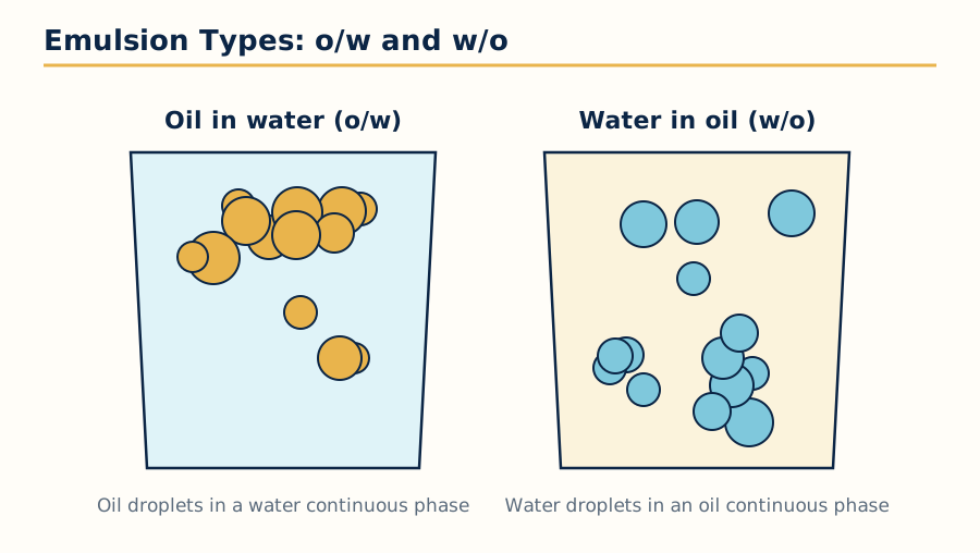 Figure: The two simple emulsion types. In an o/w emulsion the oil is the dispersed phase; in a w/o emulsion the water is dispersed in oil.
1.8 Suspensions: preparation and stability
A pharmaceutical suspension is a dispersion of insoluble solid particles in a liquid medium, used when the drug is insoluble, unstable in solution, or needed as a depot or a palatable liquid for children. Particle size is usually in the range of about 0.5 to 10 micrometres for oral products.
Preparation. The drug is first reduced to the required size and wetted with a wetting agent, then dispersed in a vehicle containing suspending agents that build viscosity and structure (for example methylcellulose, tragacanth, bentonite or carbomers). Flocculating agents, buffers, preservatives, sweeteners and flavours are added, and the product is homogenised or milled to a uniform dispersion.
Stability and the two sedimentation behaviours. Particles settle by Stokes law. What matters is how they settle:
- Deflocculated system: particles are individually dispersed and repel each other. They settle slowly, but the sediment packs tightly into a hard cake that cannot be redispersed (caking). Supernatant stays clear for long.
- Flocculated system: particles are linked in loose flocs (controlled flocculation is produced by electrolytes, surfactants or polymers that reduce the zeta potential to a chosen range). Flocs settle fast and form a loose, voluminous sediment that redisperses easily on shaking.
Controlled flocculation is therefore the preferred strategy for most suspensions: slightly less elegant settling, but the patient can always resuspend the dose uniformly. Evaluation includes sedimentation volume (the ratio of sediment height to total height, F), redispersibility, particle size, viscosity and rheology, zeta potential and drug content uniformity.
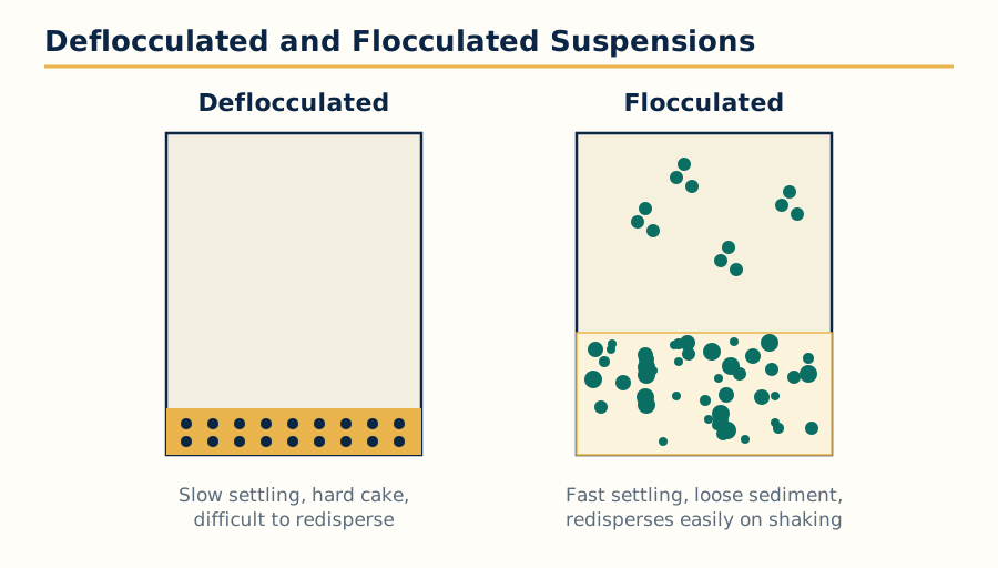 Figure: Deflocculated particles settle slowly but cake hard; flocculated particles settle fast into a loose sediment that shakes back into a uniform suspension.
1.9 SMEDDS: self-microemulsifying drug delivery systems
Many new drugs are poorly water soluble, and their oral absorption is limited by dissolution. SMEDDS are a formulation answer to this problem. A SMEDDS is an isotropic mixture of an oil, a surfactant, and usually a cosurfactant or cosolvent, with the drug dissolved in it. The mixture is filled into a soft or hard capsule as a liquid or semisolid. On contact with gastrointestinal fluid and gentle agitation, it spontaneously forms a fine oil in water microemulsion with droplets commonly below about 200 nanometres, presenting the drug in a solubilised form over a very large surface area.
Components are selected from solubility studies and phase diagrams: the oil dissolves the drug and forms the droplet core; the surfactant (often a high HLB nonionic surfactant) stabilises the droplets; the cosurfactant improves flexibility of the interfacial film and widens the self-emulsifying region. Advantages are improved dissolution and oral bioavailability of lipophilic drugs, more reproducible absorption with smaller food effects in many cases, and a simple capsule presentation. Limitations are a high surfactant load (possible gastrointestinal irritation), drug precipitation risk on dispersion or digestion, and limited drug loading. Evaluation includes self-emulsification time, droplet size and zeta potential after dispersion, robustness to dilution, precipitation studies, dissolution testing and stability of the filled capsules.
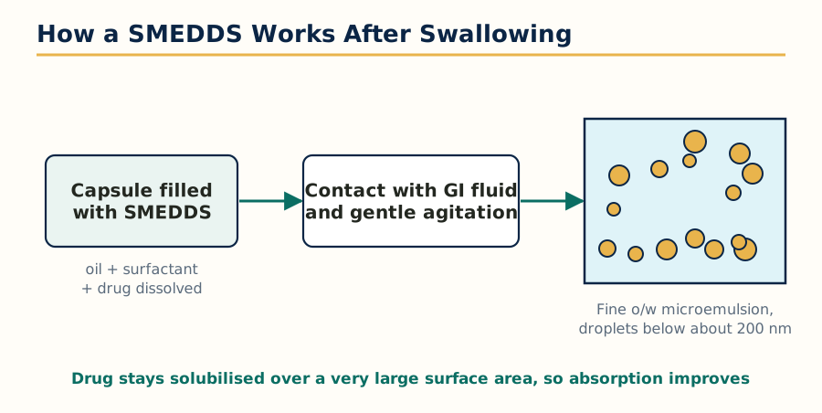 Figure: A SMEDDS capsule disperses spontaneously in gastrointestinal fluid to a fine microemulsion, keeping the drug solubilised for absorption.
1.10 Large and small volume parenterals
Parenteral products are sterile preparations given by injection or infusion. Small volume parenterals (SVP) are injections of 100 mL or less, typically ampoules, vials and prefilled syringes. Large volume parenterals (LVP) are infusions above 100 mL, typically 250 to 1000 mL of intravenous fluids, nutrition or dialysis solutions.
Physiological considerations. The product enters the body past all protective barriers, so the formulation must respect physiology: tonicity close to that of blood (isotonic, adjusted with sodium chloride, dextrose or mannitol) to avoid pain and haemolysis; pH as near physiological as buffers and drug stability allow; freedom from pyrogens (bacterial endotoxins), controlled by a strict endotoxin limit; sterility, an absolute requirement; and freedom from visible and sub-visible particulate matter, which can embolise in small vessels.
Formulation components. The vehicle is almost always Water for Injection (for LVP and for reconstitution) or a non-aqueous vehicle for a few injections. Added substances include antimicrobial preservatives (only in multidose SVP, never in LVP), antioxidants, buffers, tonicity adjusters, solubilisers and stabilisers, each justified and controlled.
Manufacturing. Production takes place in classified cleanrooms with a sterile core. In outline: preparation of Water for Injection, compounding, filtration (including sterilising grade membrane filtration at 0.22 micrometres where used), filling into washed and depyrogenated containers, sealing, terminal sterilisation by moist heat where the product allows it, or aseptic processing where it does not, then inspection for particles and container integrity. LVP in plastic containers add container forming and sealing steps.
Evaluation. Sterility testing, bacterial endotoxin testing, particulate matter counts, assay and pH, container closure integrity, extractables and leachables for plastic systems, and for LVP also volume, osmolality and clarity checks. The combination of sterility and endotoxin control is why parenterals are the most demanding products in this subject.
1.11 Optimization techniques: concept and parameters
Optimization in formulation means finding the best combination of the variables that control a product, so that the product meets all its quality targets at the same time. The classical approach, changing one factor at a time and keeping the others fixed, is slow, uses many experiments, and misses interactions between factors. Modern optimization uses planned statistical experiments to map the effect of several factors together, with far fewer runs.
The vocabulary of optimization:
- Independent variables (factors): the inputs the formulator can set, for example binder concentration, lubricant level, compression force, or the ratio of oil to surfactant in an emulsion. They are studied at chosen levels (low, middle, high).
- Dependent variables (responses): the measured outputs, for example hardness, disintegration time, dissolution at 30 minutes, viscosity or droplet size.
- Constraints: the acceptable limits on responses (for example disintegration not more than 15 minutes). A formulation is only acceptable inside its constraints.
- Optimum: the combination of factor levels that gives the most desirable set of responses within the constraints.
1.12 Statistical designs: factorial, response surface and contour methods
Factorial designs study two or more factors at two or more levels in all combinations. A 2 level factorial design with 3 factors needs 8 experiments and gives the main effect of each factor and the interactions between them, which the one factor at a time method cannot detect. Fractional factorial designs use a carefully chosen fraction of the runs for screening many factors. Factorial designs are the workhorse of formulation optimization: typical responses studied are tablet hardness and dissolution against binder and lubricant levels, or emulsion droplet size against oil and surfactant levels.
Response surface methodology (RSM) fits a mathematical model (usually a polynomial) relating the responses to the factors, using designs such as the central composite design or the Box-Behnken design, which add centre and star points to a factorial core. The fitted surface shows how the response changes across the whole experimental region, not only at the tested points, and the optimum can be read or computed from the model.
Contour designs and contour plots present the fitted surface in two dimensions: lines on the plot join factor combinations that give the same response value, like contours on a map. Overlaying the contour plots of several responses shows the region, sometimes called the design space or sweet spot, where all responses meet their constraints at once. Any formulation chosen inside that region is expected to pass.
Applications in formulation and processing. Optimization is applied to tablet formulations (binder, disintegrant and lubricant levels against hardness, friability and dissolution), granulation and compression parameters, emulsion and suspension compositions, coating processes, and analytical method development. The practical gain is a formulation that is understood, not just found: the formulator knows which factors matter, how they interact, and how much room exists before the product fails.
Optimization workflow
List factors (independent variables) and responses (dependent variables)
        |
        v
Choose a design: screening design, then factorial design
        |
        v
Prepare and test the experimental runs in random order
        |
        v
Fit models, check interactions and significance (ANOVA)
        |
        v
Draw response surfaces and contour overlays
        |
        v
Pick the optimum inside the design space, confirm with fresh batches
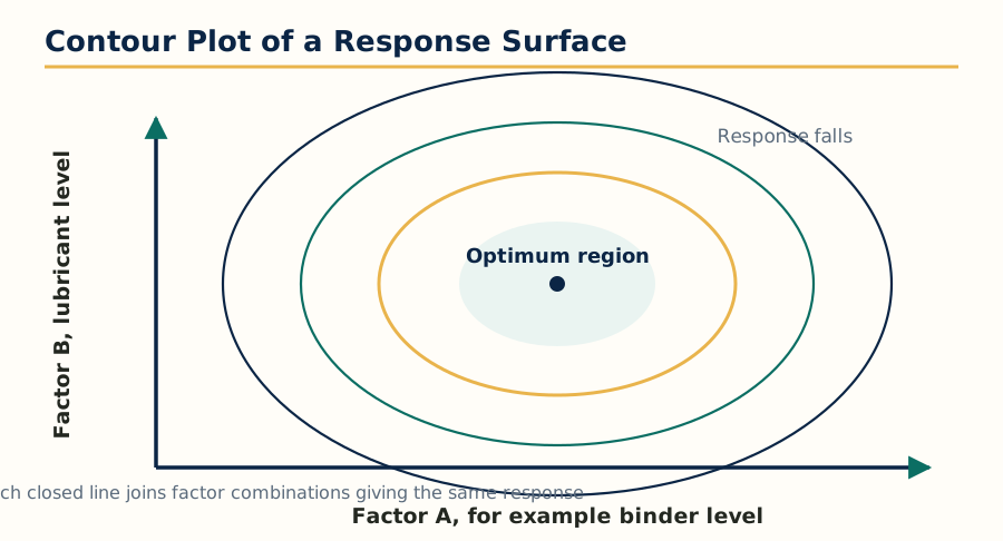 Figure: A contour plot of a fitted response surface. Overlaying such plots for several responses reveals the design space in which all responses pass.
Unit 2: Validation
2.1 Introduction to pharmaceutical validation
Validation is documented evidence that a process, equipment, system or method does what it is designed to do, consistently and reproducibly. In the words of the regulatory definition used worldwide, process validation is documented evidence that a process, operated within established parameters, can perform effectively and reproducibly to produce a product meeting its predetermined specifications and quality attributes. Validation is not testing a few finished batches and hoping they pass; it is building proof, in advance and in writing, that the process is in control.
Validation sits inside the quality system between qualification of facilities and equipment (section 2.8) and routine quality control. Qualification shows the equipment is installed and works correctly; validation shows the whole process, using that equipment and those materials, repeatedly makes a product of the required quality.
2.2 Scope and merits of validation
The scope of validation covers every part of manufacture that can affect product quality:
- Process validation: the manufacturing process itself, for each product.
- Cleaning validation: proof that cleaning procedures remove residues of product, cleaning agents and microbes to below accepted limits, so there is no cross contamination.
- Analytical method validation: proof that a test method is accurate, precise, specific and reliable for its purpose.
- Equipment and utility validation (qualification): presses, autoclaves, ovens, purified water and HVAC systems.
- Computerised system validation: software and automated systems that control or record production.
The merits of validation are practical as well as regulatory: it is required by GMP law and by every regulator; it reduces batch failures, rework and rejections; it gives a deep, documented understanding of the process, so deviations can be judged on evidence; it lowers the cost of quality because testing of finished product alone cannot detect every failure; and it makes technology transfer and scale up safer, because the critical parameters are already known.
2.3 Validation master plan and calibration master plan
The validation master plan (VMP) is the company level document that describes the whole validation programme: the philosophy and policy, the facilities, systems, equipment and processes to be validated, the responsibilities of each department, the order and priority of work, the documents to be produced (protocols and reports), and how changes and revalidation are handled. Every validation activity in the plant traces back to the VMP, and auditors ask for it early.
Calibration is the comparison of a measurement against a known standard, with adjustment or correction where needed, so that instruments read truly. The calibration master plan lists every instrument that needs calibration (balances, pressure and temperature gauges, pH meters, autoclave sensors, dissolution baths), the standard used, the frequency, the acceptance limits and the action when an instrument is found out of calibration. An uncalibrated instrument silently invalidates every result it touches, which is why calibration is planned and documented with the same discipline as validation.
2.4 ICH and WHO guidelines for calibration and validation of equipment
The ICH guidelines give the internationally harmonised framework. ICH Q7 (GMP for active pharmaceutical ingredients) and the general GMP guides require qualification and calibration programmes; ICH Q8, Q9 and Q10 add the modern lifecycle thinking: pharmaceutical development, quality risk management and the pharmaceutical quality system. ICH Q2 covers validation of analytical procedures. The WHO GMP guidelines and their supplementary guidelines on validation (including the WHO guideline on process validation and on heating, ventilation and air conditioning systems) give detailed expectations used widely by regulators in India and other countries: written protocols, predefined acceptance criteria, calibration at defined intervals with traceable standards, and documented evidence for every claim.
In practice, for equipment this means: each instrument and system is identified and listed; critical parameters are defined; calibration is done against standards traceable to national or international references; labels show calibration status and due date; and validation or qualification is performed before the equipment is used for GMP production, and repeated after major repair or relocation.
2.5 Types of validation
Process validation is classified by when it is done relative to routine production:
- Prospective validation: carried out before a new product or process is released for routine sale, on the basis of development and pilot or initial commercial batches. This is the standard and preferred type.
- Concurrent validation: carried out during routine production, in exceptional circumstances, for example where a product has a long history of good results and a justified reason exists; data are collected on actual production batches.
- Retrospective validation: based on review of historical production and testing data for a product already on the market. It is acceptable only where processes are well established and rich data exist, and its use is now limited.
- Revalidation: repetition of validation after a significant change (equipment, material source, process parameter, site) or periodically, to confirm the process remains in the validated state.
Alongside these, cleaning validation, analytical method validation and equipment qualification follow their own protocols but share the same logic: define, test against criteria, document.
2.6 Validation of specific dosage forms
The same framework is specialised for each dosage form, because the critical parameters differ:
- Tablets: validation of blending (blend uniformity), granulation end point, drying (moisture), compression (weight, hardness, friability across the run) and coating.
- Capsules: blend uniformity, fill weight control, moisture of shells.
- Liquid orals and suspensions: mixing time and order, homogeneity of sampling, preservative effectiveness and fill volume.
- Sterile products: sterilisation cycle validation (heat distribution and penetration, biological indicators), aseptic process simulation by media fill, container closure integrity and environmental monitoring.
In each case the protocol names the critical process parameters, the sampling plan, the tests and the acceptance criteria before a single batch is run; the report compares the results with the criteria and concludes whether the process is validated.
2.7 Government regulation and the manufacturing process model
Validation is a legal expectation, not a company preference. In India, the Drugs and Cosmetics Act and Rules, with Schedule M, require validated processes and equipment; the US FDA states the requirement in 21 CFR Parts 210 and 211 and in its process validation guidance, which organises validation as a lifecycle of process design, process qualification and continued process verification; the EU GMP Annex 15 does the same in Europe. Exporting companies must satisfy the strictest market they supply.
The manufacturing process model used in protocols shows the process as a chain: inputs (materials, equipment, utilities, trained people, environment) enter defined process steps with controlled parameters, and produce outputs (intermediate and finished product) that are measured against specifications. Validation studies the chain step by step: it identifies which parameters are critical to quality, sets their proven acceptable ranges, and shows by evidence that holding the parameters inside those ranges always gives an acceptable output.
2.8 Qualification of facilities: URS, DQ, IQ, OQ, PQ
New facilities and equipment pass through a documented qualification sequence before validation of products begins:
- User requirement specification (URS): the user department writes what the equipment or facility must do: capacity, performance, materials of construction, utilities, regulatory and documentation requirements. The URS is the contract against which everything else is checked.
- Design qualification (DQ): documented verification that the proposed design meets the URS and GMP requirements, done before purchase or construction is finalised.
- Installation qualification (IQ): checking and recording that the delivered equipment is installed as designed and as the manufacturer specifies: identity, components, utilities connected, manuals and drawings received, calibration of instruments started.
- Operational qualification (OQ): testing that the equipment operates within its specified ranges across its working limits, for example an oven holding temperature uniformly at its set points, or a press running at its speed range.
- Performance qualification (PQ): showing the equipment, in the real process with real materials, consistently produces the required result, for example consecutive batches meeting all specifications.
Qualification sequence for facilities and equipment
User requirement specification (URS)
        |
        v
Design qualification (DQ): design checked against URS and GMP
        |
        v
Installation qualification (IQ): installed as specified
        |
        v
Operational qualification (OQ): works across its operating ranges
        |
        v
Performance qualification (PQ): performs in the real process
        |
        v
Equipment released for process validation and routine use
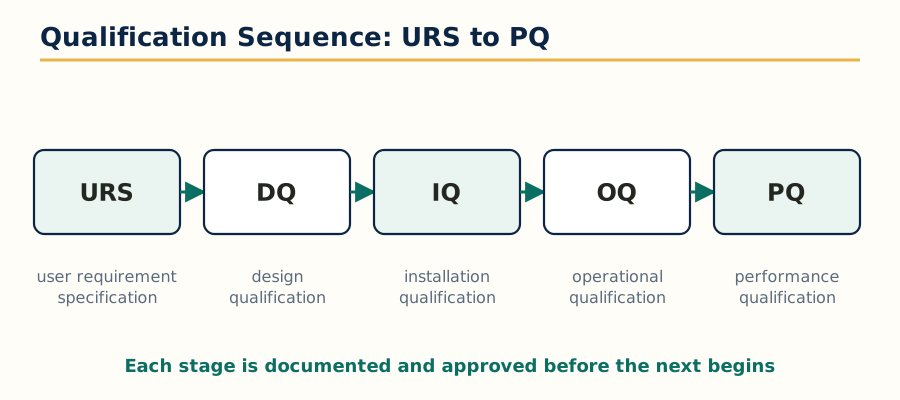 Figure: The qualification sequence for facilities and equipment: URS, DQ, IQ, OQ and PQ, each documented and approved before the next begins.
Unit 3: cGMP and Industrial Management
3.1 cGMP: objectives and policies
Current good manufacturing practice, cGMP, is the part of quality assurance that ensures products are consistently produced and controlled to the quality standards appropriate to their intended use. The word current is important: expectations rise as knowledge and technology improve, and a practice that passed inspection ten years ago may not pass today.
The objectives of cGMP are that:
- Every batch is made by defined, written procedures, by trained people, in suitable premises with suitable equipment.
- Materials are correct, tested and traceable; every step is documented as it happens, so any batch can be reconstructed from its records.
- Contamination and cross contamination are prevented; mix ups between products and labels are impossible by design.
- Deviations are recorded, investigated and corrected; complaints and recalls can be executed completely.
The policy instruments that deliver these objectives include the quality management system and its manuals, standard operating procedures (SOPs) for every operation, batch manufacturing and packaging records, training programmes, self inspection and audit, vendor qualification, and change control. Schedule M in India, WHO GMP, EU GMP and US FDA 21 CFR 210/211 are the written forms of the same policy. cGMP is a cost, but it is cheaper than recalls, regulatory action and loss of trust.
3.2 Layout of buildings
Plant layout is a GMP tool. A well laid out building separates flows so that materials, people, products and waste do not cross in ways that risk contamination or mix up. Principles include:
- Logical unidirectional flow: raw materials enter at dispensing, move through production stages to packing and the finished goods store, without back tracking.
- Separation of areas: dispensing, granulation, compression, coating and packing each in defined rooms; special segregation for potent, sensitising or beta lactam products, which need dedicated or strictly controlled facilities.
- Cleanliness grades: sterile manufacture uses graded cleanrooms (Grades A to D in EU terms) with airlocks and pressure differentials; oral solid areas use controlled, clean conditions with dust extraction.
- Construction details: smooth, impervious, easily cleaned walls, floors and ceilings; no cracks or open joints; drains designed against backflow; adequate lighting and ventilation; insect and rodent proofing.
- Supporting areas: quality control laboratories, wash areas, tool rooms, change rooms and rest areas placed so that they serve production without disturbing it.
3.3 Services and utilities
Services are the hidden systems that keep production in its validated environment:
- HVAC (heating, ventilation and air conditioning): controls temperature, humidity, air changes, filtration through HEPA filters and pressure differentials between rooms, so dust and microbes are kept out of cleaner areas.
- Water systems: purified water and Water for Injection are produced, stored and distributed in validated loops, tested chemically and microbiologically; water is the most used raw material and the most common source of contamination.
- Compressed air and gases: filtered, oil free and dry where they contact product.
- Steam and power: clean steam for sterilisation, stable power and backup for critical equipment.
Each service is qualified, monitored with defined alert and action limits, and maintained on schedule; a failed HVAC or water system stops production just as surely as a failed machine.
3.4 Equipment and their maintenance
Production equipment must be designed so it can be cleaned, does not react with or shed into the product, and can be operated and maintained safely: food grade contact materials such as stainless steel 316L, smooth welded surfaces, and no dead spaces where product can lodge. Equipment is identified with status labels (clean, in use, under maintenance), used within its qualified range, and recorded in log books.
Maintenance is planned, not improvised. Preventive maintenance schedules cover lubrication, calibration, replacement of worn parts and inspection at defined intervals, done so production plans are not disturbed; breakdown maintenance is documented and its impact on product assessed. After any significant maintenance, the equipment returns to use through cleaning, and where needed requalification, before GMP production resumes.
3.5 Production management and production organization
Production management is the planning, organising and controlling of manufacturing so that the right products are made, in the right quantity, at the right time and cost, and to the right quality. The production organisation is usually headed by a production manager or head of production, with section heads for each dosage form area, shift in charges, supervisors and operators, working with the quality assurance and quality control departments, which are independent of production. Independence of quality from production is a GMP requirement, because the department that makes a product must not be the only judge of whether it may be sold.
The core activities are setting production plans from sales forecasts and orders, scheduling machines and people, ensuring materials and documents are ready before a batch starts, monitoring output and yields, and reviewing batch records for release.
3.6 Materials management, handling and transportation
Materials management covers procurement, receipt, storage, issue and control of raw materials and packaging materials. On receipt, materials are quarantined, sampled and tested by quality control, and released or rejected before use. Stores are organised so that approved, quarantined and rejected materials cannot be mixed (status labelling and segregated areas), stock rotates by first expiry first out, and storage conditions of temperature and humidity are monitored.
Handling and transportation inside and outside the plant must protect the material: clean covered containers, protection from weather and contamination during transport, validated cold chain for temperature sensitive products, and complete documentation so every movement is traceable from supplier to finished batch.
3.7 Inventory management and control
Inventory is money sitting on shelves: too much blocks capital and risks expiry, too little stops production. Inventory control balances the two. Standard tools include:
- ABC analysis: materials are ranked by annual usage value. A items (few, high value) get tight control and frequent review; C items (many, low value) get simple control.
- VED analysis: vital, essential and desirable classification by criticality to production, combined with ABC for stocking policy.
- Economic order quantity (EOQ): the order size that minimises the sum of ordering cost and holding cost.
- Safety stock and reorder level: buffer stock held against supply delay, and the stock level at which a fresh order is placed, calculated from consumption rate and lead time.
- Perpetual inventory records: stock cards or computerised systems updated with every receipt and issue, verified by periodic physical counting.
3.8 Production planning and control
Production planning and control (PPC) converts demand into a feasible manufacturing programme. Its steps are routing (the sequence of operations for a product), scheduling (when each batch runs on which equipment), loading (matching work to machine and manpower capacity), and follow up (tracking progress, expediting delayed work, and rescheduling when deviations occur). Good PPC keeps equipment utilised without overloading it, keeps work in progress low, and protects delivery dates. In a GMP plant, PPC must also respect cleaning and changeover times, campaign rules and validation status: a plan that ignores a mandatory cleaning between products is not a plan, it is a deviation waiting to happen.
3.9 Sales forecasting, budget and cost control
Sales forecasting estimates future demand from past sales, market trends, seasonality and planned promotions; it drives the production plan, material procurement and manpower planning. Errors in forecast become either stock outs or expired stock, so forecasting is a shared duty of sales, production and planning.
A budget is the financial expression of the plan: expected sales, production costs (materials, labour, overheads), and capital spending for a period. Cost control compares actual costs with the budget and with standard costs, investigates variances, and acts on them, for example by reducing wastage of materials, improving yields, controlling overtime and energy use, and negotiating purchase prices. Yield reconciliation of every batch is where budget control and GMP meet: unexplained loss is both a cost problem and a quality signal.
3.10 Industrial and personnel relations
Industrial relations is the relationship between management, workers and their unions. In a pharmaceutical plant, good relations are a quality issue as well as a human one: trained, stable and motivated staff make fewer errors. The essentials are clear communication, fair wages and working conditions under the applicable labour laws, grievance handling procedures, worker participation through committees, and disciplined but respectful supervision. Personnel management in the GMP sense adds: defined job descriptions, training on SOPs and hygiene before a person works in production, documented training records, health checks for staff in sterile and production areas, and strict gowning and hygiene discipline. A person who does not understand why a rule exists will break it under pressure; training is therefore a cGMP activity, not an optional extra.
3.11 Concept of total quality management
Total quality management (TQM) is a management philosophy in which quality is the responsibility of every person in the organisation, and the goal is continuous improvement of processes to achieve complete customer satisfaction. Its main ideas are:
- Customer focus: the patient and the prescriber are the final customers; internal departments treat the next process step as their customer too.
- Continuous improvement (kaizen): small, constant improvements by everyone, rather than occasional large changes.
- Employee involvement: quality circles and suggestion schemes use the knowledge of the people who run the process.
- Process approach and data based decisions: problems are solved by measuring and analysing the process, using the statistical tools of Unit 5 of this subject.
- Prevention over inspection: building quality into the product and process rather than testing it in at the end.
TQM contains GMP rather than replacing it: GMP gives the non-negotiable legal floor of quality, and TQM adds the culture and the improvement engine on top of it.
Unit 4: Compression and Compaction
4.1 Physics of tablet compression
Tableting converts a powder or granulation into a compact of definite shape, strength and weight by applying pressure between two punches inside a die. The physics of this event decides the quality of every tablet: its hardness, friability, disintegration and dissolution. The process on a rotary press runs in stages:
- Die filling: the lower punch drops and the die fills with a measured volume of feed from the hopper, usually with the help of a feed frame. Fill uniformity decides weight uniformity.
- Metering and pre-compression: the lower punch rises to the exact fill position, excess feed is removed, and on many presses a small pre-compression force removes entrapped air.
- Main compression: the upper punch enters the die and the punches move towards each other, applying the main force; the powder consolidates into a tablet.
- Decompression and ejection: the upper punch withdraws, the pressure releases (the compact relaxes slightly, called elastic recovery), and the lower punch rises to push the tablet out of the die, where it is swept away.
A tablet press records force against time or punch travel; these traces are the raw material of sections 4.5 and 5.5.
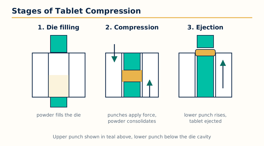 Figure: The stages of one compression cycle on a tablet press: die filling, compression, then decompression and ejection.
4.2 Compression and consolidation: what happens inside the die
As pressure rises, the powder bed consolidates in a recognisable sequence of mechanisms:
- Particle rearrangement: at low pressure, particles slide and rotate into the voids, and packing density rises with little true deformation. Fine particles fill gaps between coarse ones.
- Elastic deformation: particles deform reversibly; the deformation disappears when pressure is removed and contributes to elastic recovery.
- Plastic deformation: beyond the yield point, particles flow permanently into new shapes, greatly increasing the area of contact between them. Materials such as microcrystalline cellulose consolidate mainly this way.
- Fragmentation (brittle fracture): hard, brittle materials such as lactose and dicalcium phosphate break into smaller pieces, creating fresh, clean surfaces that bond well; fragmentation is largely independent of compression speed.
- Bonding: the enlarged, closely pressed surfaces bond by intermolecular forces (van der Waals), by solid bridges formed where local heat or pressure causes fusion, and by mechanical interlocking. The total bonded area, created by deformation and fragmentation, is what gives the tablet its strength.
Consolidation is the sum of these mechanisms. Whether a material prefers plastic flow or fragmentation explains its behaviour: plastic materials are sensitive to lubrication and to press speed (less time to flow gives weaker tablets), while brittle materials are more forgiving of both. Most formulations mix the two types deliberately.
4.3 Effect of friction
Friction acts at two places. Interparticle friction between particles resists their movement during rearrangement; die wall friction, between the compact and the die wall, is the bigger practical problem. As the upper punch pushes down, the die wall friction opposes the movement, so the force reaching the lower part of the compact is less than the applied force. Consequences:
- Uneven density: the top of the tablet is denser than the bottom, worst in tall, thin compacts; this can cause capping and lamination on ejection.
- High ejection force: the tablet must be pushed out against the friction of the die wall; a large residual radial force makes ejection hard and can score or break tablets.
- Heat and wear: friction converts work into heat, warming punches and dies and accelerating tooling wear.
Lubricants such as magnesium stearate reduce die wall friction by forming a film on the die wall and on particle surfaces. The price of lubrication is bonding interference: the same film coats particle surfaces and weakens tablet strength, especially in plastic materials, and excessive lubricant or over mixing slows wetting and dissolution. Antiadherents and glidants handle related problems: sticking to punch faces and poor powder flow respectively. Managing friction is therefore a balance: enough lubricant to eject cleanly, never so much that the tablet weakens.
4.4 Distribution of forces
Force applied by the upper punch is not transmitted perfectly through the compact. The ratio of the force measured at the lower punch to the force applied at the upper punch is called the force transmission ratio (or R value). In a perfectly lubricated, frictionless system it would be 1; in practice it is reduced by die wall friction, and it is a sensitive measure of lubrication quality: values above about 0.9 indicate a well lubricated system.
Within the compact, stress exists in two directions: axial stress along the punch movement, and radial stress pressing the compact against the die wall. During compression the radial pressure rises with the axial pressure; at the end of decompression a residual radial pressure remains, which is what makes ejection force necessary. The radial pressure also explains elastic recovery behaviour and the splitting tendency of tablets: while axial pressure is released fully when the upper punch leaves, the compact is still squeezed radially inside the die, and sudden release of this stress at ejection can split weak compacts. Measurement of upper and lower punch forces, ejection force and residual radial pressure, using instrumented presses and instrumented dies, is the experimental base for all compaction science in this unit and the next.
4.5 Compaction profiles
A compaction profile is a recorded relationship during the compression cycle that converts the event into data. The common profiles are:
- Force time profile: force plotted against time through one cycle; shows the rise, dwell and fall of pressure and detects sticking or irregular feeding.
- Force displacement profile: force plotted against punch travel or punch separation. The area under the curve is the work of compression, and its shape separates the work used in consolidation from the work returned as elastic recovery during decompression. Comparing profiles of formulations shows which one consolidates easily and which wastes energy on friction or elasticity.
- Pressure porosity (density) profile: the relative density of the compact plotted against applied pressure (often in logarithmic form), summarising how a material densifies; it is the parent plot of the Heckel analysis of Unit 5.
- In-die thickness and recovery measurements: the thickness of the compact under load and after ejection, giving elastic recovery directly.
Profiles are used to compare materials and formulations, to select lubricant levels, to detect over pressing (where extra force adds no strength, only capping risk) and to transfer a process between presses by matching profiles rather than only machine settings.
4.6 Solubility
Solubility is the maximum amount of a solute that dissolves in a given amount of solvent at a given temperature, forming a saturated solution. In pharmaceutics it is usually expressed for the drug in water or in buffer at body temperature, in mg per mL or as descriptive terms from practically insoluble to freely soluble. Solubility matters in this subject at two points: a drug must dissolve before it can be absorbed, so aqueous solubility and dissolution rate together limit bioavailability for most oral products; and within the tablet, the solubility of the drug and of excipients influences consolidation behaviour and what happens when the compact meets liquid: a soluble filler such as lactose dissolves at the surface and aids disintegration and release, while an insoluble matrix holds its structure.
Factors affecting solubility include the nature of the drug crystal (polymorphs differ in solubility, with metastable forms more soluble and less stable), particle size (smaller particles dissolve faster and very fine particles are slightly more soluble), temperature, pH for ionisable drugs (a weak base dissolves better at low pH; salts of weak acids and bases are chosen to exploit this), and the presence of solubilising agents. The pH solubility profile and the salt form of a drug are therefore decided in preformulation (Unit 1), and revisited here because they decide whether a compressed tablet can deliver its drug into solution at all.
Unit 5: Consolidation Parameters, Dissolution Models and Pharmaceutical Statistics
5.1 Consolidation parameters: the study framework
Consolidation parameters are the measured quantities that describe how a powder responds to pressure and how the resulting compact performs. Unit 4 described the mechanisms; this unit covers the numbers: parameters that describe the compacting process itself (transmitted force, ejection force, work of compression, elastic recovery), parameters that describe release from the compact or dosage form (diffusion and dissolution parameters), pharmacokinetic parameters that link the profile in the test tube to the profile in the body, and the model plots (Heckel, Higuchi, Peppas) and comparison factors (f1 and f2) built from them. The statistics at the end of the unit are the tools used to decide whether observed differences are real.
5.2 Diffusion parameters
Diffusion is the movement of molecules from a region of high concentration to one of low concentration under a concentration gradient. Fick's first law states that the flux (amount crossing unit area per unit time) is proportional to the concentration gradient: J = minus D dC/dx, where D is the diffusion coefficient. Fick's second law describes how concentration changes with time at any point. In dosage forms, diffusion controls release through polymer membranes and matrices, and permeation across biological membranes.
The practical diffusion parameters are the diffusion coefficient D (which falls as viscosity rises and as molecule size grows), the permeability coefficient of a membrane (which combines D with the partition coefficient and membrane thickness), the lag time before steady state flux is reached, and the steady state flux itself. For a reservoir system with a rate controlling membrane, flux is nearly constant, giving zero order release; for a matrix, the diffusing front moves and the release follows the Higuchi square root pattern of section 5.7.
5.3 Dissolution parameters
Dissolution is the process by which a solid drug enters solution; for most oral products it must happen before absorption. The Noyes-Whitney equation describes the rate: dC/dt = (D A / h) times (Cs minus C), where D is the diffusion coefficient, A the surface area of the solid, h the thickness of the stagnant diffusion layer around each particle, Cs the saturation solubility and C the concentration already in solution. The equation explains every common way of speeding dissolution: reduce particle size (A rises), stir better (h falls), choose a more soluble form (Cs rises), and keep sink conditions (C stays low).
Dissolution parameters reported for a product include the percentage released at specified times (for example Q at 30 or 45 minutes), the dissolution efficiency (area under the dissolution curve up to a time, expressed as a percentage of the rectangle for complete release), the mean dissolution time, and t50 percent, the time for half the drug to dissolve. Whole profiles, not single points, are compared when formulations change, using the similarity approach of section 5.6.
5.4 Pharmacokinetic parameters in profile comparison
Pharmacokinetic parameters translate the in vitro profile into the expected behaviour in the body. The standard parameters are Cmax (the peak plasma concentration), Tmax (the time to reach the peak) and AUC, the area under the plasma concentration time curve, which measures the total extent of absorption. When a modified release product is developed or a formulation changes, these parameters from bioequivalence studies are compared with the reference product: the rate of absorption is judged by Cmax and Tmax, the extent by AUC. The pharmacokinetic parameters are the end point that the diffusion and dissolution parameters of the earlier sections are trying to predict, and correlations between dissolution and absorption (in vitro in vivo correlations) are built on exactly this chain.
5.5 Heckel plots
The Heckel plot is the standard analysis of compaction data. As pressure P increases, the relative density D of the compact rises towards 1. Heckel proposed the relation: ln [1 / (1 minus D)] = k P + A, where k is a constant related to the plasticity of the material and A is an intercept reflecting the initial rearrangement and packing. A plot of ln [1/(1-D)] against P typically has three regions:
- Region 1, initial curve: at low pressure the line curves upward; particles rearrange and fragment, and density rises faster than the straight line predicts.
- Region 2, straight line portion: plastic deformation dominates. The slope k is inversely related to the yield pressure of the material: the reciprocal 1/k is the mean yield pressure, Py. A low Py (steep slope) means a soft, plastic material that consolidates easily; a high Py means a hard, resistant material.
- Region 3, upper curve: at high pressure the line bends again as the compact approaches its limiting density, work hardens, and elastic effects grow.
Heckel plot (shape)
ln[1/(1-D)]
   |                                  ______ Region 3: hardening
   |                             ____/
   |                        ____/   Region 2: straight line
   |                   ____/        slope k, Py = 1/k
   |              ___--
   |          __--   Region 1: rearrangement
   |      ___--
   |_____--________________________________ applied pressure P
Heckel analysis compares materials and the effect of lubricants, moisture and press speed on Py, and it quantifies the difference between plastic and fragmenting behaviour. Deviations of a plot from the usual shape warn of problems such as over lubrication or capping tendency.
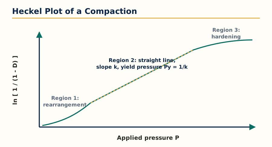 Figure: The Heckel plot. The straight line region gives the slope k, and the mean yield pressure is Py equals 1 over k.
5.6 Similarity factors f1 and f2
When a formulation, process or site changes, regulators ask whether the new dissolution profile matches the reference. The similarity approach answers with two numbers calculated from the mean percentage dissolved of reference (R) and test (T) products at the same time points:
- Difference factor f1: the average percentage difference between the two profiles. f1 = [ sum of |Rt minus Tt| divided by sum of Rt ] times 100. Profiles are considered similar when f1 lies between 0 and 15.
- Similarity factor f2: a logarithmic measure of closeness: f2 = 50 times log of { [1 + (1/n) sum (Rt minus Tt) squared] raised to minus 0.5, times 100 }. Profiles are considered similar when f2 lies between 50 and 100; f2 = 100 means identical profiles.
Conditions for a valid comparison include: the same dissolution conditions and time points for both products, at least 3 to 4 time points, 12 units of each product, only one time point after both products have reached 85 percent dissolved, and limited variability (coefficient of variation not more than 20 percent at the early points and 10 percent later). The f2 approach is preferred worldwide because it judges the whole profile rather than single points.
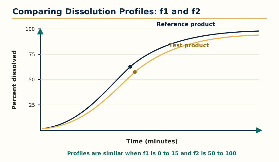 Figure: Reference and test dissolution profiles compared point by point; the pair is similar when f1 is 0 to 15 and f2 is 50 to 100.
5.7 Higuchi and Peppas plots
The Higuchi model describes drug release from an insoluble matrix in which the drug is dispersed. Its central result is that the amount of drug released is proportional to the square root of time: Q = kH times the square root of t. A plot of cumulative release against the square root of time (the Higuchi plot) is a straight line when release is controlled by diffusion through the matrix as the depletion zone moves inward. Higuchi release is expected from matrix tablets, ointments and transdermal systems in which a solid drug reservoir is dispersed in the vehicle.
The Korsmeyer-Peppas (power law) model is a general equation for the first 60 percent of release: Mt/M infinity = k t raised to the power n. Taking logarithms gives a straight line plot of log fraction released against log time, whose slope is the release exponent n. The value of n identifies the mechanism:
| Geometry | n for Fickian diffusion | n for anomalous (mixed) transport | n for Case II (relaxation controlled) |
|---|---|---|---|
| Thin film (slab) | 0.5 | 0.5 to 1.0 | 1.0 |
| Cylinder | 0.45 | 0.45 to 0.89 | 0.89 |
| Sphere | 0.43 | 0.43 to 0.85 | 0.85 |
An exponent at the Fickian value means release is diffusion controlled; an intermediate value means diffusion and polymer relaxation or erosion both contribute; the upper value means constant rate, relaxation or erosion controlled release. Fitting the Higuchi and Peppas models to the same data set is a routine part of release mechanism work.
5.8 Linearity, standard deviation and the concept of significance
Before any test of significance, the quality of the measurement itself is described.
Linearity is the ability of an analytical method to give results directly proportional to the concentration of the analyte over a stated range; it is shown by the calibration plot and its correlation. In statistics generally, linearity also refers to whether a relationship between two variables follows a straight line, which decides which model may be fitted (as in the Heckel and Peppas plots above).
Standard deviation (SD) measures the spread of results around their mean. A small SD means tight, reproducible data; a large SD means scatter. The variance is the square of the SD, and the coefficient of variation (SD divided by the mean, times 100) expresses spread as a percentage, allowing comparison between measurements of different size.
Concept of significance: a difference between two sets of results is statistically significant when it is larger than could reasonably arise from random variation alone. The judgement is made by choosing a significance level, most commonly 5 percent (p less than 0.05): if the probability of seeing a difference at least this large, when there is really no difference, is below 5 percent, the difference is declared significant. Significance is not importance: with enough data, a trivially small difference becomes significant, so statistical results are always read together with their practical size.
5.9 Chi square test, Student's t test and ANOVA
These three tests answer the three most common questions in pharmaceutical data work:
| Test | Question it answers | Typical pharmaceutical use |
|---|---|---|
| Chi square test | Do observed frequencies differ from expected frequencies? | Goodness of fit; association in categorical data, for example pass and fail counts between two processes |
| Student's t test | Do the means of two groups differ significantly? | Comparing mean assay or hardness of two formulations; paired t test for before and after on the same units |
| ANOVA (analysis of variance) | Do the means of three or more groups differ, and which factors matter? | Comparing several formulations at once; analysing factorial design experiments of Unit 1, separating the effects of factors and their interactions |
Chi square test compares counts in categories. The statistic sums, over all categories, (observed minus expected) squared divided by expected. A large chi square value means the observed counts stray too far from expectation to be chance. Conditions: data must be counts, categories independent, and expected frequencies should not be too small.
Student's t test compares means using the t statistic, the difference of means divided by the standard error of the difference. It exists in unpaired form (two independent groups) and paired form (the same units measured twice, tested on the differences). Assumptions are approximately normal data and, for the simple form, similar variances.
ANOVA extends the t test to many groups and many factors at once, without the error inflation that repeated t tests cause. It divides the total variation in the data into parts due to each factor, due to interactions, and due to random error (the residual). An F test on each factor compares its mean square with the error mean square: a large F with a small p value means the factor genuinely affects the response. ANOVA is the analysis engine behind the factorial and response surface designs used for optimization, closing the loop of this subject: experiments are designed statistically, products are made under validated, GMP controlled conditions, and the results are judged with these tests.
Frequently Asked Questions
Q: What is the aim of preformulation studies? Preformulation characterises the physicochemical properties of a drug, alone and with excipients, before a dosage form is designed. It covers solubility, stability, crystal form, particle properties and excipient compatibility, and its results decide the dosage form, the excipients, the process and the packaging, saving far greater cost if problems appear later.
Q: How are drug excipient interactions detected? A combination of methods is used. DSC gives a rapid thermal screen (shifts or loss of the drug melting peak suggest interaction), infrared spectroscopy checks for changes in characteristic peaks, isothermal stress testing of mixtures imitates storage and shows physical change, and HPLC gives the final proof by quantifying actual degradation products.
Q: What is t90 and how is it calculated for a first order reaction? t90 is the shelf life time at which the drug concentration falls to 90 percent of its initial value, the usual acceptable potency limit. For a first order reaction, t90 equals 0.105 divided by the rate constant k. The related half life is t1/2 equals 0.693 divided by k, independent of the starting concentration for first order reactions.
Q: What are the stability study conditions under ICH guidelines? Long term studies run at the zone condition (for Zone IV countries such as India, 30 degrees Celsius at 65 or 75 percent relative humidity) over the full shelf life, and accelerated studies run at 40 degrees Celsius and 75 percent relative humidity for 6 months. Stress testing exposes the drug substance to severe heat, light, oxidation and hydrolysis to reveal degradation pathways.
Q: What is the difference between a flocculated and a deflocculated suspension? In a deflocculated suspension the particles are separate, settle slowly, but pack into a hard cake that cannot be redispersed. In a flocculated suspension the particles form loose flocs that settle quickly to a loose, voluminous sediment which redisperses easily on shaking. Controlled flocculation is preferred for most pharmaceutical suspensions.
Q: What is the difference between validation and qualification? Qualification applies to facilities and equipment: it proves through URS, DQ, IQ, OQ and PQ that the equipment is designed, installed and works as intended. Validation applies to processes and methods: it proves with documented evidence that the whole process consistently produces product meeting its specifications.
Q: What do IQ, OQ and PQ mean? Installation qualification checks that equipment is delivered and installed as specified. Operational qualification tests that it operates correctly across its working ranges. Performance qualification shows that, in the real process with real materials, it consistently gives the required result, after which the equipment can be released for process validation and routine production.
Q: What is a factorial design and why is it better than changing one factor at a time? A factorial design studies two or more factors at two or more levels in all combinations, in a planned set of experiments. Unlike the one factor at a time approach, it detects interactions between factors, where the effect of one factor depends on the level of another, and it reaches the optimum with fewer, better organised experiments.
Q: What is a Heckel plot and what does the slope tell us? A Heckel plot graphs ln of 1 over (1 minus relative density) against applied pressure. Its straight line region reflects plastic deformation; the slope k is inversely related to the mean yield pressure, Py equals 1 over k. A low yield pressure indicates a soft, easily consolidated plastic material, while a high yield pressure indicates a hard material that resists consolidation.
Q: When are two dissolution profiles considered similar? Profiles are similar when the difference factor f1 lies between 0 and 15 and the similarity factor f2 lies between 50 and 100, calculated from mean percentage dissolved values of 12 units of each product at the same time points under the same conditions, with only one time point included after both products pass 85 percent dissolved.
Complete MPH103T notes, all 5 units in one PDF, free to keep.
Other M.Pharm subjects: MPH101T · MPC101T · MPL101T · MPH102T · MPH103T · MPH104T · M.Pharm