
MPH202T — Advanced Biopharmaceutics and Pharmacokinetics
4 hrs/week, 4 credits, 60 hours, 100 marks (75 end semester + 25 sessional). Notes follow the M.Pharm syllabus, unit by unit.
MPH202T Advanced Biopharmaceutics and Pharmacokinetics notes for M.Pharm Semester 2 Pharmaceutics: GI absorption, dissolution and IVIVC, compartment models, nonlinear kinetics, bioavailability and bioequivalence, biotechnology drug kinetics, with free unit wise PDF downloads on PharmacoLearn.
Units in this subject
- Unit 1 — Drug Absorption from the Gastrointestinal Tract
- Unit 2 — Biopharmaceutic Considerations in Drug Product Design and In Vitro Drug Product Performance
- Unit 3 — Pharmacokinetics
- Unit 4 — Drug Product Performance, In Vivo: Bioavailability and Bioequivalence
- Unit 5 — Application of Pharmacokinetics
Download MPH202T PDF Notes
Free PDFs for this subject, one per unit:
Advanced Biopharmaceutics and Pharmacokinetics, subject code MPH202T, is a core Semester 2 subject of M.Pharm Pharmaceutics. It carries 4 credits and 60 hours of theory, taught at 4 hours per week, for 100 marks.
Biopharmaceutics studies how the drug's physicochemical properties, its dosage form and the body's physiology together decide how much drug reaches the systemic circulation, and how fast. Pharmacokinetics describes, in numbers, what the body does to the drug (absorption, distribution, metabolism, excretion) and turns plasma data into parameters such as clearance, volume of distribution and half life used to calculate doses and regimens. The first unit follows a drug through the gastrointestinal tract: the mechanisms by which it crosses the gut wall, the pH-partition theory, dissolution and the Noyes-Whitney equation, and the modern transport model built on permeability, solubility and charge state. The second unit turns to drug product design and in vitro performance: the factors that make one formulation perform better than another, dissolution and drug release testing, and in vitro-in vivo correlation. The third unit is the mathematical core: compartment models for intravenous bolus, intravenous infusion and extravascular administration, the two compartment model, nonlinear pharmacokinetics with the Michaelis-Menten equation, and drug interaction mechanisms. The fourth unit measures drug product performance in vivo: bioavailability, bioequivalence and its crossover designs, the biopharmaceutics classification system, permeability methods and biosimilars. The last unit applies all of it to modified release products, targeted delivery and the biotechnology products (proteins, monoclonal antibodies, oligonucleotides, vaccines, gene therapies), whose behaviour follows the same principles with new complications. A student who completes this subject should be able to derive pharmacokinetic parameters from raw data, judge the quality of a dissolution or bioequivalence study, and use pharmacokinetic reasoning to design and evaluate a dosage regimen.
Unit 1: Drug Absorption from the Gastrointestinal Tract
1.1 The gastrointestinal tract as the site of absorption
The oral route is the most used route because it is convenient, safe and cheap, and the gastrointestinal tract (GIT) is built for absorption: a long tube whose surface is enormously amplified. The small intestine is the principal site. Its wall is folded (folds of Kerckring), the folds carry villi, and each epithelial cell carries microvilli, the brush border. Together these multiply the small intestinal surface to roughly 200 square metres, against a plain tube area of less than one square metre.
The regions differ in ways that matter. The stomach is mainly a mixing and holding organ with a thick mucus layer, a small surface and a strongly acidic lumen (pH about 1.2 to 2 fasting); most drugs are absorbed only weakly there despite the pH favourable to weak acids, because the surface is small. The small intestine (duodenum, jejunum, ileum) has a luminal pH rising from about 6 to about 7.4, the huge surface above, bile and pancreatic secretions, and a residence time of about 3 to 4 hours: it is where the great majority of oral absorption happens. The colon has a smaller surface, no villi, viscous contents and a large bacterial population; it matters for colonic delivery and for sustained release products whose remaining dose reaches it. Gastric emptying controls the rate at which drug is presented to the small intestine, so for most immediate release products gastric emptying, not the crossing of the gut wall, sets the pace of absorption: fatty food delays emptying, while liquids and small particles empty faster.
Absorption is a chain of steps: the dosage form must disintegrate, the drug must dissolve and survive acid and enzymes in the lumen and gut wall, and it must cross the epithelial cell layer. The slowest step is the rate limiting step, an idea that returns in Unit 2.
1.2 Mechanisms of drug absorption
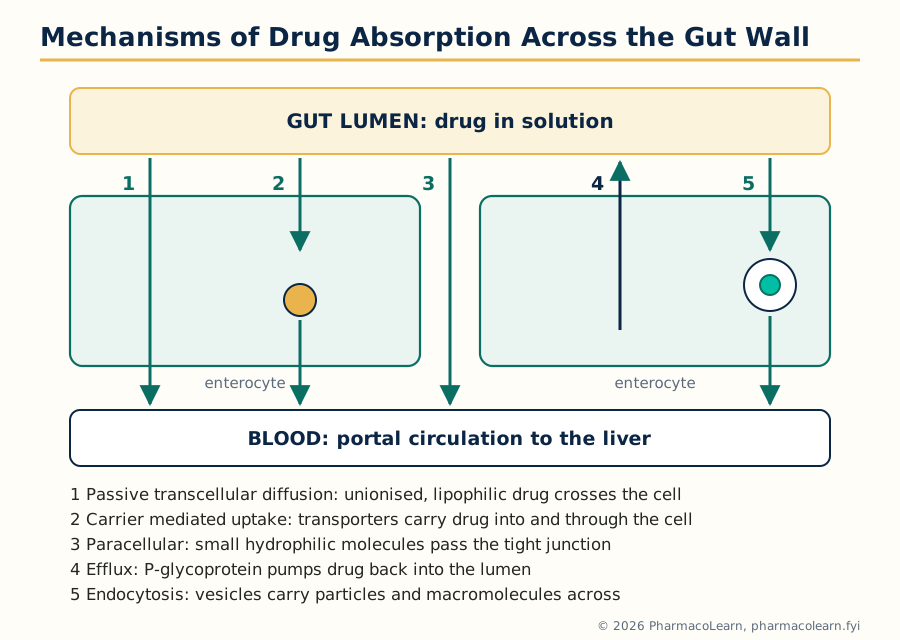 Figure: The routes by which a drug molecule can cross the intestinal epithelium. Passive transcellular diffusion carries most marketed drugs; the other routes matter for specific drug classes and are targets of modern formulation design.
A drug can cross the intestinal epithelium by several mechanisms, and a real drug often uses more than one.
- Passive diffusion (transcellular). The drug partitions from the aqueous lumen into the lipid cell membrane, diffuses across the cell and partitions out into the blood. No energy or carrier is involved, the rate is proportional to the concentration gradient and to lipid solubility, and the process is not saturable. This is the route of most small, moderately lipophilic drugs, and the route the pH-partition theory (section 1.3) describes.
- Paracellular transport. The drug passes between the cells, through the tight junctions that seal the epithelial sheet. The aqueous pores are narrow (a few angstroms), so this route is restricted to small hydrophilic molecules and contributes little for most drugs, but it is the only passive route available to very polar compounds. Section 1.13 returns to the tight junction complex.
- Carrier mediated transport. Membrane proteins carry specific substrates: facilitated diffusion moves the drug down its concentration gradient without energy; active transport moves it against the gradient at the cost of ATP or an ion gradient. Uptake transporters carry some drugs and drug-like nutrients: PEPT1 carries beta-lactam antibiotics and valaciclovir, and amino acid and glucose transporters carry look-alikes (L-DOPA, gabapentin). Carrier mediated absorption is saturable, so the fraction absorbed can fall as dose rises, and it is subject to competition and inhibition, a source of drug interactions (Unit 3).
- Efflux transport. Other membrane proteins pump drug back into the lumen. P-glycoprotein (P-gp), breast cancer resistance protein (BCRP) and related efflux transporters sit on the luminal (apical) membrane of the enterocyte and eject absorbed molecules, working with the metabolising enzyme CYP3A4 inside the cell as a first pass barrier in the gut wall. Efflux limits the bioavailability of drugs such as digoxin, ciclosporin and many anticancer agents, and inhibiting it raises their blood levels.
- Endocytosis and transcytosis. Cells take up particles and macromolecules in vesicles (pinocytosis for fluid, phagocytosis for particles, receptor mediated endocytosis for ligands) and, in some cells, carry them across. Quantitatively minor for conventional drugs, but the entry route exploited in research for oral delivery of peptides, nanoparticles and vaccines.
- Ion pair transport and pore transport. A highly ionised drug can cross as a neutral ion pair with an oppositely charged ion; very small molecules (below about 150 to 200 in molecular weight, such as urea) can pass through water filled membrane pores. Both are minor routes listed for completeness.
The balance of uptake and efflux transporters, with passive permeability, decides the permeability term of the transport model in section 1.12.
1.3 The pH-partition theory of drug absorption
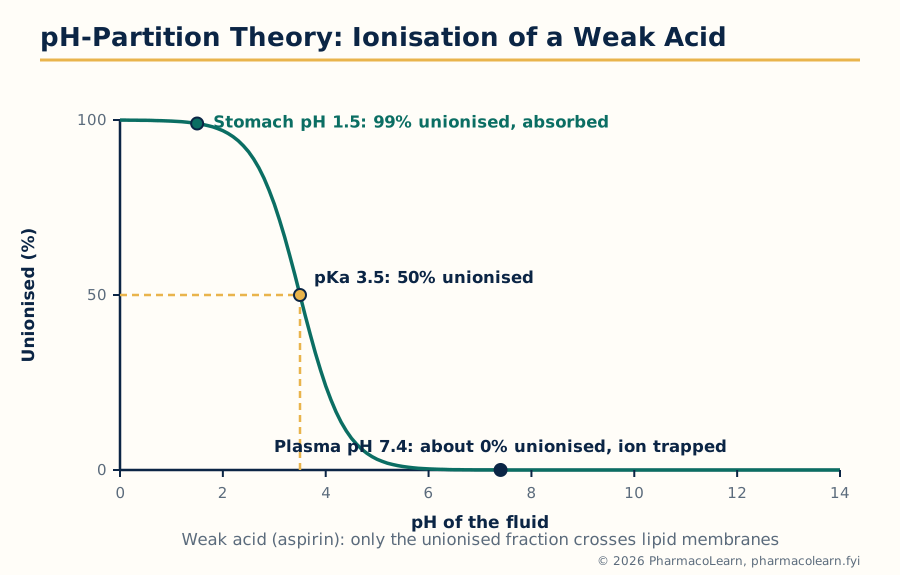 Figure: The pH-partition idea in one picture: membranes pass the unionised species, so the ionisation set by local pH decides how much drug is available to cross, and ionisation on the far side traps it there.
Most drugs are weak acids or weak bases, existing in solution as a mixture of ionised and unionised molecules whose proportions are set by the fluid pH and the drug's pKa. The pH-partition theory states that the lipid membrane is permeable essentially only to the unionised species, so absorption is fastest where pH makes the drug mostly unionised: a weak acid in acid, a weak base in alkali. The Henderson-Hasselbalch equations give the proportions:
- For a weak acid: pH = pKa + log([ionised] / [unionised])
- For a weak base: pH = pKa + log([unionised] / [ionised])
Worked example. Aspirin is a weak acid with pKa 3.5. In fasting gastric fluid at pH 1.5, the ratio ionised to unionised is 10 raised to (1.5 - 3.5), that is 0.01: about 99 percent of the aspirin is unionised and available to cross membranes. In plasma at pH 7.4 the ratio is 10 raised to (7.4 - 3.5), about 7900: aspirin reaching the blood is almost completely ionised, and because the ionised form crosses back only very slowly, it is effectively trapped in the plasma.
The theory is a useful first approximation, not the whole truth, and its limitations are standard examination material:
- It predicts that weak acids should be absorbed mainly from the stomach, yet in practice most are absorbed mainly from the small intestine, whose surface area and blood flow outweigh the less favourable pH. pH sets the fraction available to cross; area and time decide how much actually crosses.
- The ionised species is not completely impermeable; it crosses slowly by the paracellular route and through pores, so even highly ionised drugs show some absorption.
- The pH at the membrane surface is not the bulk luminal pH: an acidic microclimate exists at the intestinal surface (section 1.13).
- The theory ignores transporters and dissolution. A drug that is unionised but undissolved is not absorbed at all.
1.4 Factors affecting drug absorption
The factors fall in three groups. Physiological factors include gastric emptying rate (usually the pacing step for immediate release forms), intestinal motility and transit time, gastrointestinal pH and its change with food, disease and age, blood flow to the gut, food (which can delay, reduce or occasionally increase absorption, for example by stimulating bile), gut wall and hepatic first pass metabolism, and the bacterial flora metabolising some drugs in the colon. Physicochemical factors include aqueous solubility, dissolution rate, pKa and the resulting ionisation at gut pH, lipid solubility (partition coefficient), particle size and surface area, the solid state form, and chemical stability in gut fluids. Formulation factors cover the dosage form type (sections 1.7 to 1.10), the excipients, and manufacturing variables such as compression force and coating. A useful rule: absorption fails if any one of dissolution, stability or permeation fails, and improving the factor that is not rate limiting changes nothing.
1.5 Dissolution and the Noyes-Whitney equation
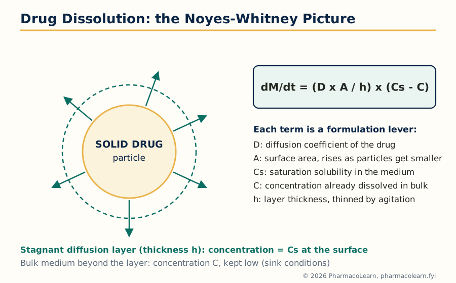 Figure: Dissolution as Noyes and Whitney pictured it: a thin stagnant layer saturated at Cs surrounds the particle, and diffusion across that layer is the slow step that the equation describes.
A solid drug cannot cross the gut wall; it must first dissolve. Dissolution is the process by which drug molecules leave the solid surface and enter solution, and for poorly soluble drugs it is the rate limiting step of the whole absorption chain. It has two steps: molecules detach from the crystal surface into a thin, stagnant saturated layer around the particle (the diffusion layer, of thickness h), then diffuse from this layer into the bulk fluid, where the concentration is lower. Diffusion across the stagnant layer is the slow step, which is why the Noyes-Whitney equation is a form of Fick's law:
dM/dt = (D x A / h) x (Cs - C)
where dM/dt is the rate of dissolution (amount per unit time), D the diffusion coefficient in the medium, A the surface area of solid exposed, h the diffusion layer thickness, Cs the saturation solubility (the concentration in the stagnant layer) and C the bulk concentration at time t. Dividing by the medium volume V gives dC/dt = (D x A / (V x h)) x (Cs - C).
Two ideas follow directly. First, under sink conditions, when the bulk concentration stays low (conventionally below about 10 to 20 percent of Cs) because dissolved drug is removed, by absorption in the body or by a large medium volume in vitro, the term (Cs - C) stays nearly equal to Cs and the dissolution rate is nearly constant. Second, every factor in the equation is a lever for the formulator: the rate rises in proportion as the factors change. Section 1.6 takes the factors one by one.
1.6 Factors affecting the dissolution rate
- Surface area and particle size. Rate is proportional to A, so reducing particle size (micronisation, and in modern practice nanosizing) is the oldest and most reliable way to speed dissolution of a poorly soluble drug; griseofulvin is the classic example whose bioavailability roughly doubled on micronisation. Very fine powders can aggregate and float, so wetting agents may be needed to realise the area.
- Solubility (Cs). Rate is proportional to Cs. A salt of a weak acid or base usually dissolves faster than the free form because it creates a surface pH favourable to its own dissolution; a metastable polymorph or the amorphous form has a higher apparent solubility than the stable crystal, at the price of a risk of converting back.
- Diffusion layer thickness (h). Agitation thins the layer: faster stirring or faster gut motility increases the rate, which is why dissolution results depend on stirring speed and why the method must control it (Unit 2).
- Diffusion coefficient (D). D falls as medium viscosity rises, so viscous vehicles and gel forming excipients slow dissolution; D falls with molecular size.
- Temperature and medium. Solubility and D rise with temperature; medium pH changes Cs directly for ionisable drugs, so dissolution media mimic gastric or intestinal pH.
- Wetting. A hydrophobic powder surface traps air and reduces the effective area; surfactants and hydrophilic excipients improve wetting and raise the rate.
1.7 Role of the dosage form: solutions
A solution (including elixirs, hydroalcoholic solutions, and syrups, concentrated sugar solutions) contains the drug already dissolved, so the dissolution step is absent and the drug is available for absorption as soon as it reaches the intestine. Solutions therefore usually give the fastest onset and highest bioavailability of the oral forms, and are the reference against which other forms are judged. Their disadvantages are practical: chemical stability is poorer (hydrolysis is fastest in solution), taste masking is difficult, doses are bulky and less precisely measured, and precipitation can occur if the drug is near its solubility limit when diluted or when its pH changes in the gut. For a solution, absorption is governed by gastric emptying and membrane permeation alone, so the ranking of oral forms by absorption speed usually begins: solution, then suspension, then capsule, then tablet, with coated and sustained release forms slowest of all.
1.8 Role of the dosage form: suspensions
A suspension is a dispersion of fine solid drug particles in a liquid vehicle. Dissolution is present, but because the drug is already divided into small particles with a large surface area, it is usually fast, and suspensions are absorbed nearly as quickly as solutions and clearly faster than tablets of the same drug. Their biopharmaceutic risks are particle growth on storage (crystal growth and caking change A and therefore the dissolution rate), poor redispersion if the bottle is not shaken, and dose non-uniformity. The particle size distribution of a suspension is a critical quality attribute for exactly the reason the Noyes-Whitney equation gives: it sets A.
1.9 Role of the dosage form: capsules
A capsule is a dose of drug (powder, granules or pellets) in a gelatin shell. On contact with gut fluid the shell hydrates, softens and ruptures within minutes, releasing contents that behave much like a powder or suspension. Capsules therefore absorb at rates between suspensions and tablets. The variables that matter are the filling (loose powder disaggregates freely; a plug formed under pressure behaves more like a tablet), the excipients (a hydrophilic diluent such as lactose aids wetting; a little disintegrant helps the plug break up), and the shell, which must be stored so it does not cross link and dissolve slowly, a known cause of failed dissolution in aged capsules. Soft gelatin capsules carry the drug dissolved or dispersed in a liquid fill, which for poorly soluble lipophilic drugs can approach the performance of a solution.
1.10 Role of the dosage form: tablets
The tablet is the most used and most engineered oral form, with the longest chain of steps before absorption: it must disintegrate into granules, the granules must deaggregate into primary particles, and only then can the drug dissolve. Each step adds time and variability, so tablets usually show the slowest and most variable absorption of the immediate release forms, and tablet formulation is largely the art of keeping those steps fast: disintegrants (starch, croscarmellose, sodium starch glycolate), a soluble diluent, lubricant kept at the minimum level (excess hydrophobic lubricant such as magnesium stearate coats particles and slows wetting and dissolution), and compression force high enough for strength but not so high that disintegration slows. Coatings add their own delay: film coats rupture quickly, enteric coats deliberately prevent release until the tablet leaves the stomach, sugar coats add bulk and time.
1.11 Dissolution methods and the correlation of in vitro with in vivo data
Because dissolution is the gatekeeper step for solid forms, in vitro dissolution testing is the standard laboratory method for predicting and controlling it: the form sits in a measured volume of medium at 37 degrees Celsius under defined agitation, and samples over time build a profile. The apparatus and discipline of the test are Unit 2 material; the point here is what the test is for. It should rank formulations in the same order as the body does. The correlation of in vivo data with in vitro dissolution data rests on the idea that, when dissolution is rate limiting in vivo, the fraction dissolved in vitro should track the fraction absorbed in vivo, formalised as IVIVC in Unit 2 (section 2.9).
1.12 Transport model: permeability, solubility and charge state
The pH-partition theory is an older idea built on one property, lipid solubility. The modern transport model, developed largely by Avdeef and reflected in the reference list of this subject, describes intestinal absorption through three properties of the molecule, measured together:
- Permeability: the rate at which the molecule crosses a membrane model, measured in artificial membrane systems (PAMPA) or cell monolayers (Caco-2, section 4.9), combining passive transcellular, paracellular and transporter contributions.
- Solubility: the amount that can dissolve, measured as a function of pH across the gastrointestinal range, since an ionisable drug's solubility differs at every pH.
- Charge state: the distribution of ionisation states at each pH, worked out from the pKa values. Charge state links the other two: it sets solubility at each pH (ionised species are more soluble) and permeability at each pH (the unionised species permeates best), so the two pH profiles slope in opposite directions and the pH of best absorption is a compromise.
The pH partition hypothesis survives inside this model: the intrinsic permeability of the unionised species is the ceiling value, from which effective permeability at any pH follows by weighting by the fraction unionised.
1.13 Properties of the GIT that shape the transport model
Three properties of the tract itself complete the picture. First, the pH gradient: luminal pH rises from about 1.2 to 2 in the fasting stomach, through about 6 in the duodenum, to about 7.4 in the ileum and falls slightly in the colon, so a travelling molecule meets changing charge state and solubility, and weak bases dissolving in the stomach may precipitate in the intestine. Second, the pH microclimate: the mucosal surface carries an unstirred water layer and a microclimate whose pH (about 5.3 to 6.1 in the jejunum) is more acidic than the bulk luminal pH. A drug is absorbed from this microclimate, so its ionisation at the membrane is set by the microclimate pH: one reason weak acids are absorbed from the intestine better than bulk pH predicts. The intracellular pH environment (about 7.0 to 7.2 inside the enterocyte) then sets the ionisation of whatever has crossed the apical membrane, contributing to ion trapping and to the behaviour of intracellular enzymes and efflux transporters. Third, the tight junction complex: tight junctions, protein complexes (claudins, occludin, junctional adhesion molecules) joining the cells near their apical surface, seal the paracellular space, fence off the apical from the basolateral membrane, and are dynamically regulated. They restrict the paracellular route of section 1.2 to very small hydrophilic molecules, and safely modulating them is an active strategy for delivering peptides.
The absorption chain, and where this unit's ideas act
Tablet or capsule
   |  disintegration and deaggregation (dosage form, Unit 1 sections 1.7 to 1.10)
   v
Solid drug particles
   |  dissolution: Noyes-Whitney, proportional to A and (Cs - C) (sections 1.5, 1.6)
   v
Drug in solution in gut fluid
   |  permeation: pH-partition, transporters, tight junctions (sections 1.2, 1.3, 1.12, 1.13)
   v
Portal blood, then liver (first pass metabolism), then systemic circulation
Unit 2: Biopharmaceutic Considerations in Drug Product Design and In Vitro Drug Product Performance
2.1 Introduction: drug product performance begins in vitro
A drug product performs in two arenas. In vitro performance is what the laboratory measures before any patient is involved: disintegration, dissolution and release, content uniformity, stability. In vivo performance, bioavailability and bioequivalence, is Unit 4. This unit covers the in vitro side and the design thinking connecting the two, because in vivo performance is largely decided by the in vitro properties built in.
2.2 Biopharmaceutic factors affecting drug bioavailability and the rate limiting steps
Bioavailability, the rate and extent to which the active drug reaches the systemic circulation, is the product of surviving every step between the mouth and the blood. The biopharmaceutic factors can be read straight off the absorption chain of Unit 1:
- Release and dissolution from the dosage form. If the drug does not leave the form and dissolve, nothing else matters (sections 1.5, 1.6 and formulation).
- Stability in the gastrointestinal fluids. Acid labile drugs (penicillins, erythromycin, omeprazole) are destroyed in the stomach unless protected; lumen and gut wall enzymes digest peptides.
- Permeation of the gut wall. Set by permeability and charge state (section 1.12) and by efflux transporters.
- First pass metabolism. Drug absorbed from most of the gut passes through the liver via the portal vein before the systemic circulation; gut wall and liver enzymes (CYP3A4 above all) can remove a large fraction on this first pass, as with propranolol, verapamil and midazolam.
For any given product, one of these steps is the slowest, the rate limiting step, and only improvements to that step improve bioavailability. For a soluble, permeable drug, gastric emptying is often rate limiting; for a poorly soluble drug (the majority of new drug candidates), dissolution is rate limiting and particle size, solid form and formulation decide performance; for a soluble but poorly permeable drug, membrane permeation is rate limiting and no dissolution improvement helps; for a drug with extensive first pass metabolism, formulation can do little and dose or route must change. Identifying the rate limiting step correctly is the first act of rational drug product design, and it is the idea the biopharmaceutics classification system of Unit 4 formalises.
2.3 Physicochemical nature of the drug
The properties of the drug substance that the designer must know, and can sometimes change, are:
- Aqueous solubility and its pH profile. Solubility sets Cs in the Noyes-Whitney equation and, with the dose, whether the dose can dissolve in the available gut fluid at all.
- pKa and ionisation. Sets charge state at every gut pH, hence the balance of solubility and permeability (section 1.12), and the feasibility of salt formation.
- Partition coefficient (log P, and log D at a stated pH). A measure of lipid solubility: too low and the membrane is a barrier, too high and the drug will not dissolve in water or leave the membrane. Most orally absorbed drugs sit in a moderate range.
- Particle size and surface area. Direct control of dissolution rate (section 1.6).
- Solid state form. Polymorphs differ in solubility and stability; the stable form is the least soluble. The ritonavir episode, in which a new, less soluble polymorph appeared during production and forced the product off the market for reformulation, is the standing warning that solid form is a performance variable, not an academic detail.
- Chemical stability. Degradation in acid, solution, or by oxidation sets shelf life and may demand enteric protection.
- Salt form. The salt of an ionisable drug changes solubility, dissolution rate, stability, hygroscopicity and processability at once; salt selection is standard early development work.
2.4 Formulation factors affecting drug product performance
On the formulation side, performance is moved by the diluent (soluble lactose aids wetting and dissolution; insoluble diluents do not), the binder and granulation method (wet granulation gives dense granules that may dissolve more slowly than a direct compression blend), the disintegrant type, level and placement (inside the granules, outside them, or both), the lubricant (hydrophobic lubricants retard wetting, and over-mixing one into a blend is a classic cause of slow dissolution), surfactants and wetting agents (improving wetting, and solubilising drug in micelles), viscosity modifying agents, the coating, and the process itself: compression force, and for capsules the fill and shell condition.
2.5 Dissolution and drug release testing: compendial methods
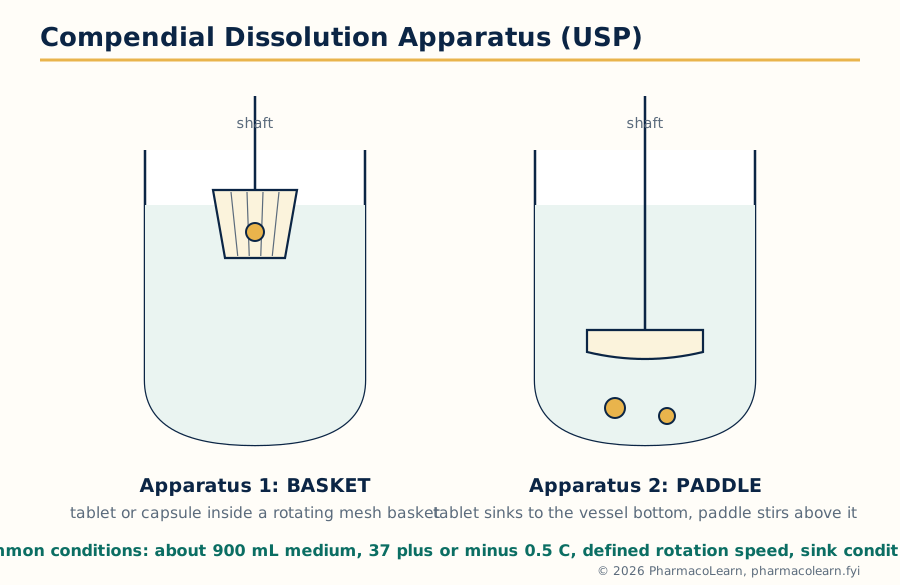 Figure: The two workhorse compendial apparatus. The basket holds the dosage form in a rotating wire mesh cage; the paddle stirs the vessel with the dosage form resting at the bottom. Every other variable, volume, temperature, speed, sampling, is fixed by the monograph.
Dissolution testing is an official quality control test described in the pharmacopoeias (USP, IP, BP, EP) with standardised apparatus. Common conditions are a medium (usually 500 to 1000 mL of water, buffer or dilute acid, mimicking gut fluid and maintaining sink conditions) at 37 plus or minus 0.5 degrees Celsius, defined agitation, defined sampling times and a validated assay. The compendial apparatus are:
| Apparatus | Name | Typical use |
|---|---|---|
| USP 1 | Rotating basket | Capsules, floating products, beads; typically 50 to 100 rpm |
| USP 2 | Paddle | Tablets and capsules (with a sinker if the form floats); typically 50 to 75 rpm; the most used apparatus |
| USP 3 | Reciprocating cylinder | Products needing changing pH media, beads and modified release forms |
| USP 4 | Flow-through cell | Poorly soluble drugs, implants, powders; medium flows continuously so sink conditions are easy |
| USP 5 | Paddle over disk | Transdermal patches |
| USP 6 | Rotating cylinder | Transdermal patches |
| USP 7 | Reciprocating holder | Transdermal and other non-disintegrating products |
Drug release testing is the same idea applied to non-oral and modified release products, where the form is designed to release over hours and the test runs correspondingly longer with multiple sampling points. For modified release products the profile itself (amount released at several times, with limits at each) is the specification, not a single time point.
2.6 Alternative methods of dissolution testing
The compendial apparatus are compromises, and several alternative or supplementary methods exist for problems they handle badly. The flow-through cell suits poorly soluble drugs because fresh medium continuously restores sink conditions. Biphasic dissolution places an organic layer (for example octanol) over the aqueous medium so dissolved drug partitions continuously into it, mimicking absorption removing drug and maintaining sink. Biorelevant media (fasted and fed state simulated intestinal fluids, FaSSIF and FeSSIF, with bile salts and lecithin) imitate the gut rather than the buffer bottle, and serve development and IVIVC building rather than routine quality control. Intrinsic dissolution measures the rate from a compressed disk of pure drug of constant area, isolating the drug property from the formulation, a characterisation tool.
2.7 Meeting dissolution requirements
A monograph states the requirement as a Q value: the percentage of labelled amount that must dissolve at the stated time (for example, Q = 80 percent at 45 minutes). Because single units vary, compliance is judged in stages against the pharmacopoeial acceptance table:
- Stage 1 (S1): test 6 units. Each unit must dissolve not less than Q + 5 percent.
- Stage 2 (S2): if S1 fails, test 6 more. The average of all 12 units must be not less than Q, and no unit may be less than Q minus 15 percent.
- Stage 3 (S3): if S2 fails, test 12 more. The average of all 24 units must be not less than Q, not more than 2 units may be less than Q minus 15 percent, and no unit may be less than Q minus 25 percent.
The staged design balances two risks: rejecting a good batch because of one odd unit, and accepting a genuinely poor batch. Meeting the requirement is a property of the whole distribution of units, not of the average alone, so formulation work aims at a mean comfortably above Q with a small spread, not at a mean exactly at Q.
2.8 Problems of variable control in dissolution testing
Dissolution is a sensitive test, and much laboratory discipline is controlling variables that have nothing to do with the product: mechanical variables (shaft wobble, vessel centring, paddle or basket height, vibration, worn baskets with clogged or distorted mesh), medium variables (dissolved air forming bubbles on tablets and baskets, so media are deaerated where the monograph requires; pH drift; temperature gradients between vessels), dosage form behaviour (a tablet that floats, sticks to the vessel wall, or cones, accumulating as a mound under the paddle where agitation is weakest), sampling variables (probe position, filter adsorption of drug, and sample volumes changing later concentrations if not corrected), and analytical variables (assay drift, standard preparation). The mirror lesson for design: robust formulations tolerate small changes in these variables; knife edge formulations do not.
2.9 In vitro-in vivo correlation (IVIVC)
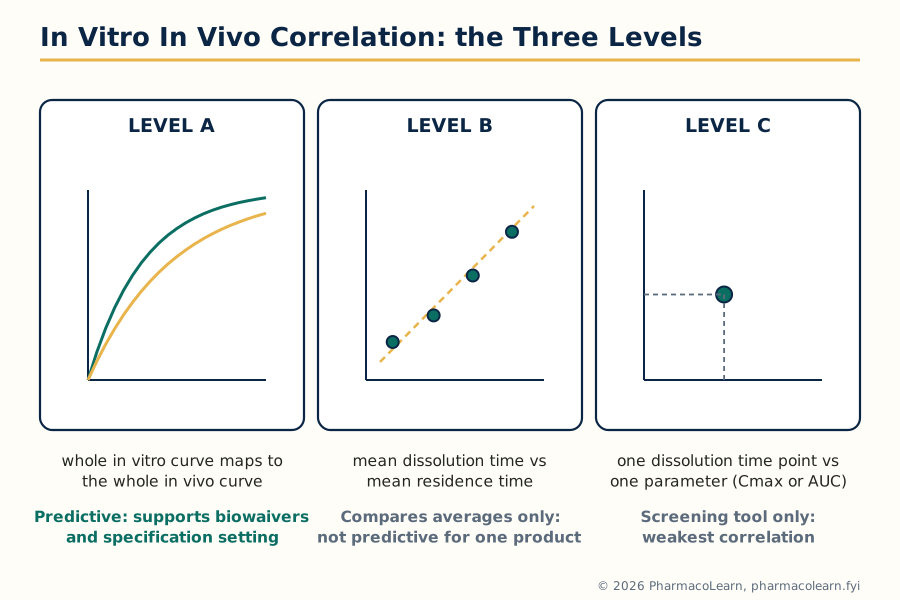 Figure: The IVIVC levels ranked by what they relate and by predictive strength. Only Level A, a point to point relation across the whole profile, can substitute for in vivo studies across the life of a product.
An IVIVC is a mathematical relationship between an in vitro property of the dosage form, usually its dissolution profile, and the in vivo response, usually the plasma profile or the fraction absorbed. Four levels are recognised, in decreasing strength:
- Level A: a point to point relationship between the in vitro dissolution curve and the in vivo input (fraction absorbed) curve, usually obtained by deconvolution of the plasma data. The whole in vitro curve maps to the whole in vivo curve, so any dissolution profile can be converted into a predicted plasma profile. This is the only level accepted as a full surrogate for bioequivalence in changes to modified release products.
- Level B: relates mean in vitro dissolution time to a mean in vivo quantity (mean residence time or mean absorption time). It uses all the data but collapses each curve to one number, so different profiles with the same mean look identical; it cannot alone justify major changes.
- Level C: relates one dissolution time point (for example percent dissolved at 2 hours) to one parameter (for example Cmax or AUC). Useful in early development for screening; too weak for regulatory substitution.
- Multiple Level C: relates one pharmacokinetic parameter to the amount dissolved at several time points; stronger than C, still short of A.
A correlation can only exist when dissolution is rate limiting in vivo; for rapidly dissolving immediate release products absorbed under permeation or gastric emptying control, Level A correlation is generally not achievable (section 2.2).
2.10 Dissolution profile comparisons
When a formulation changes (a scale up, a site transfer, a modified release redesign), the first question is whether its dissolution profile still matches the reference profile. The standard model independent comparison uses two numbers calculated from the mean profiles at matched time points:
- Difference factor f1 = [ sum of |Rt - Tt| over all time points / sum of Rt ] x 100, where Rt and Tt are the percentages dissolved of reference and test at time t. Profiles are similar when f1 is 0 to 15.
- Similarity factor f2 = 50 x log10{ [1 + (1/n) x sum of (Rt - Tt) squared] raised to minus 0.5 x 100 }, where n is the number of time points. Profiles are similar when f2 is between 50 and 100.
Worked example. Reference profile at 10, 20, 30 and 45 minutes: 30, 50, 70, 85 percent. Test profile: 32, 52, 68, 83 percent. The differences are 2, 2, 2 and 2 percent, so the sum of absolute differences is 8 and the sum of Rt is 235, giving f1 = 8/235 x 100 = 3.4. For f2, each squared difference is 4, the mean over 4 points is 4, so f2 = 50 x log10(100 / square root of 5) = 50 x log10(44.72) = 50 x 1.65 = 82.5. Since f1 (3.4) is below 15 and f2 (82.5) is above 50, the profiles are declared similar. The rules of use matter as much as the formulas: use mean profiles from 12 units, matched time points, only one time point after both profiles pass 85 percent dissolved, and respect variability limits, because f2 from noisy or mismatched points is meaningless. Very rapidly dissolving products (both profiles at or above 85 percent in 15 minutes) are accepted as similar without calculation.
2.11 Drug product stability
A drug product must perform not only on the day it is made but on the last day of its shelf life, so stability is a design property, not an afterthought. The designer considers chemical stability (hydrolysis, oxidation, photolysis, interactions with excipients, for example the reaction of amine drugs with reducing sugars), physical stability (polymorph conversion, capsule shell cross linking that slows dissolution, suspension crystal growth, emulsion creaming), and microbiological stability for liquid and semi solid products. Packaging is part of the formulation for stability purposes: moisture barrier blisters, desiccants, amber containers, nitrogen filling. Stability is proven by long term and accelerated storage studies testing assay, degradation products and, importantly here, dissolution: a product whose assay is unchanged but whose dissolution has slowed on storage has lost performance an assay alone would not reveal.
2.12 Considerations in the design of a drug product
The design logic of the unit, in order: define the target profile (route, onset, duration, dose frequency); characterise the drug (section 2.3); identify the rate limiting step (section 2.2); choose the dosage form and formulation strategy attacking that step (salt, particle size, solubilisation, protection from acid or enzymes); develop an in vitro test measuring the controlling property and, where possible, a correlation linking it to in vivo behaviour (sections 2.5 to 2.10); and set specifications and a stability programme (sections 2.7, 2.11) holding the product at its designed performance for its whole life at production scale.
Design logic of Unit 2, in one view
Target profile (onset, duration, dose)
        |
        v
Drug properties: solubility, pKa, permeability, stability, dose
        |
        v
Rate limiting step identified (dissolution? permeation? first pass?)
        |
        v
Formulation strategy attacks that step
        |
        v
In vitro test measures the controlling property (dissolution, release)
        |
        v
IVIVC or profile comparison links in vitro to in vivo
        |
        v
Specifications and stability programme hold the performance
Unit 3: Pharmacokinetics
3.1 Basic considerations: describing what the body does to the drug
Pharmacokinetics is the quantitative study of ADME: absorption, distribution, metabolism and excretion of a drug, followed through its concentration in the body over time. In practice the concentration is measured in plasma (or blood or serum), because plasma can be sampled repeatedly and, for most drugs, tracks the concentration at the site of action with a short delay. Plotting plasma concentration against time gives the plasma level time curve, and this unit extracts standard parameters from that curve and uses them to design dosage regimens.
The parameters used throughout the unit, each defined once here:
- Cmax: the peak plasma concentration after a dose.
- Tmax: the time at which Cmax occurs; a measure of the rate of absorption.
- AUC: the area under the plasma concentration time curve (concentration x time, for example mg·h/L); the measure of total drug exposure.
- C0: the concentration at time zero obtained by extrapolating the curve after an intravenous bolus; used to calculate Vd.
- K (also written Ke or kel): the overall elimination rate constant (per hour); the fraction of drug in the body eliminated per unit time.
- Half life (t1/2): the time for plasma concentration (or amount) to fall by half; for first order elimination, t1/2 = 0.693 / K.
- Volume of distribution (Vd): the apparent volume that would contain the total amount of drug in the body at the measured plasma concentration: Vd = amount in body / plasma concentration. A proportionality constant, not a real anatomical volume; a large Vd means extensive tissue distribution.
- Clearance (CL): the volume of plasma cleared of drug per unit time (for example L/h); CL = K x Vd, and for an intravenous dose CL = Dose / AUC.
- Bioavailability (F): the fraction of the administered dose that reaches the systemic circulation unchanged; Unit 4 is devoted to it.
Two kinetic orders govern almost everything. In first order (linear) kinetics, a constant fraction of drug is eliminated per unit time: K and half life are constant, and AUC rises in proportion to dose. In zero order kinetics, a constant amount is eliminated per unit time because the eliminating machinery is saturated; ethanol is the familiar example, and section 3.8 treats saturable elimination properly. Most drugs at therapeutic doses follow first order kinetics, so the models of sections 3.3 to 3.6 are built on first order rate constants.
3.2 Pharmacokinetic models
A model is a mathematical picture of the body simple enough to calculate with and realistic enough to predict. Three families are used:
- Compartment models. The body is represented as one or more compartments: not real organs, but volumes in which the drug is assumed to mix instantly and uniformly, connected by first order transfer rate constants. The mammillary model, a central compartment (blood and well perfused tissues) connected to peripheral compartments (poorly perfused tissues), is the standard picture. Sections 3.3 to 3.6 develop these.
- Physiological (flow) models. Compartments correspond to real organs with real blood flows and tissue partition coefficients. They predict real tissue concentrations and scale between species, but need much measured data and are research tools, not this subject's working model.
- Model independent description. AUC, Cmax, Tmax and half life read directly from the measured curve without assuming a compartment structure; this is how bioequivalence data (Unit 4) are compared, since the comparison must not depend on a model being right.
3.3 The one compartment model: intravenous bolus
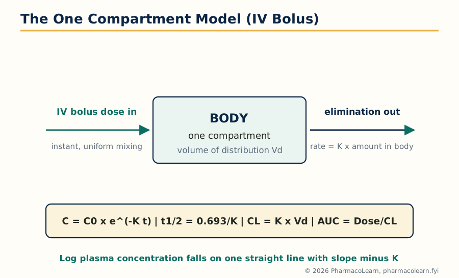 Figure: The simplest useful picture of the body: one instantly mixing volume, one first order exit. The log concentration plot is a straight line whose slope is minus K, the single most used graphical method in pharmacokinetics.
The one compartment open model treats the body as a single volume Vd into which an intravenous bolus is injected and mixes instantly, giving C0 = Dose / Vd, and from which drug is eliminated by a first order process with rate constant K. The concentration at time t is:
C = C0 x e^(-K t)
Taking logarithms gives log C = log C0 - (K / 2.303) x t, so a plot of log concentration against time is a straight line: the slope gives K, the intercept gives C0, and from these every other parameter follows: t1/2 = 0.693 / K, Vd = Dose / C0, AUC = C0 / K (the total area from zero to infinity), and CL = K x Vd = Dose / AUC.
Worked example. A 1000 mg intravenous bolus gives an extrapolated C0 of 50 mg/L and, from the log plot slope, K = 0.15 per hour.
- Vd = Dose / C0 = 1000 / 50 = 20 L.
- t1/2 = 0.693 / 0.15 = 4.62 hours.
- AUC = C0 / K = 50 / 0.15 = 333 mg·h/L.
- CL = Dose / AUC = 1000 / 333 = 3.0 L/h. Check: K x Vd = 0.15 x 20 = 3.0 L/h. The two routes to clearance agree, as they must.
- Concentration at 6 hours: C = 50 x e^(-0.15 x 6) = 50 x e^(-0.9) = 50 x 0.407 = 20.3 mg/L.
This calculation is the foundation of dose work: a loading dose is target C x Vd, and maintenance requirements are set by clearance.
3.4 The one compartment model: intravenous infusion
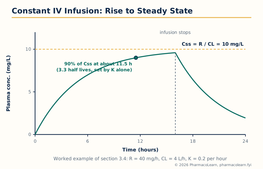 Figure: An infusion adds drug at a constant rate while elimination removes it in proportion to concentration. The two balance at the steady state, Css, and the half life alone decides how long the approach takes.
With a constant infusion rate R (amount per unit time) into the one compartment model, drug enters at a constant rate and leaves at a rate proportional to concentration, so concentration rises and levels off when input and output are equal. During the infusion:
C = (R / CL) x (1 - e^(-K t))
The plateau value is the steady state concentration, Css = R / CL. Its decisive properties are examination favourites: Css depends only on the infusion rate and the clearance, not on Vd; but the time to reach the plateau is set by the half life alone, about 50 percent of Css in one half life, 90 percent in 3.32 half lives, and practical steady state in 4 to 5 half lives. Changing the infusion rate changes the plateau but not the time taken to reach it. When the infusion stops, the concentration falls exponentially with the same K, from Css.
If the plateau must be reached immediately, a loading dose comes first: LD = Css x Vd fills the volume to the target concentration at once, after which the infusion replaces what elimination removes.
Worked example. A drug with K = 0.2 per hour and Vd = 20 L (so CL = K x Vd = 4 L/h) is infused at R = 40 mg/h.
- Css = R / CL = 40 / 4 = 10 mg/L.
- t1/2 = 0.693 / 0.2 = 3.47 hours, so the infusion reaches 90 percent of Css after 3.32 x 3.47, about 11.5 hours, and practical steady state in about 14 to 17 hours.
- Loading dose for an immediate 10 mg/L: LD = 10 x 20 = 200 mg.
- Doubling the infusion to 80 mg/h doubles Css to 20 mg/L, but it still takes the same 11.5 hours to reach 90 percent of the new plateau.
This separation, clearance sets the level and half life sets the timing, also governs repeated oral dosing, where the average steady state concentration is Css,avg = (F x Dose) / (CL x dosing interval).
3.5 The one compartment model: extravascular administration
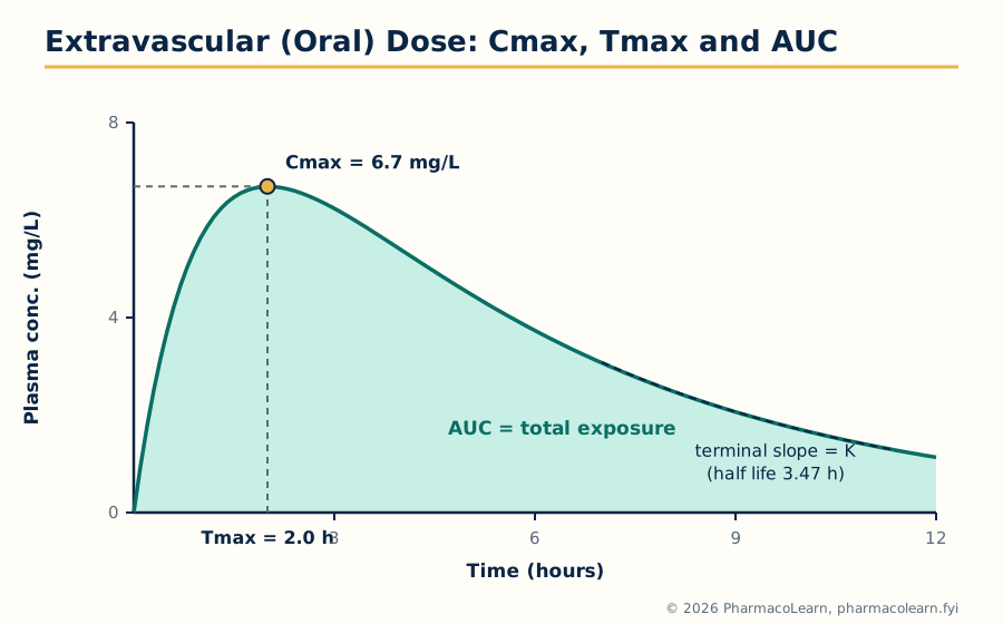 Figure: After an oral dose the curve is the sum of two exponentials: absorption pushing concentration up, elimination pulling it down. Cmax and Tmax sit at the balance point; the terminal slope gives K and the back extrapolated line gives the absorption rate constant ka.
After an oral (extravascular) dose, drug must be absorbed before it can be eliminated, and the concentration reflects both processes at once. With first order absorption (rate constant ka) and first order elimination (K), the one compartment equation is:
C = [F x Dose x ka / (Vd x (ka - K))] x (e^(-K t) - e^(-ka t))
where F is the fraction absorbed intact (bioavailability). The curve rises while absorption outruns elimination, peaks at Cmax when the two rates are momentarily equal, then declines. Tmax depends on both rate constants:
Tmax = ln(ka / K) / (ka - K)
The terminal (log linear) part of the curve has slope minus K, provided absorption has finished; extrapolating this line back and subtracting it from the measured concentrations (the method of residuals, or feathering) gives a second straight line whose slope is minus ka. One caution governs interpretation: the terminal slope reflects the slower of the two processes. Normally ka exceeds K and the terminal slope is K; but if absorption is slower than elimination (ka less than K), as with sustained release products, the terminal slope measures ka instead, the flip-flop situation, and a naive reading reports the absorption half life as if it were the elimination half life.
Worked example. A 100 mg oral dose, F = 1, Vd = 10 L, ka = 1.0 per hour, K = 0.2 per hour.
- The coefficient F x Dose x ka / (Vd x (ka - K)) = (1 x 100 x 1.0) / (10 x 0.8) = 12.5 mg/L.
- Tmax = ln(1.0 / 0.2) / (1.0 - 0.2) = ln 5 / 0.8 = 1.609 / 0.8 = 2.0 hours.
- Cmax = 12.5 x (e^(-0.2 x 2.0) - e^(-1.0 x 2.0)) = 12.5 x (0.670 - 0.135) = 12.5 x 0.535 = 6.7 mg/L.
- AUC = F x Dose / CL, with CL = K x Vd = 0.2 x 10 = 2 L/h, so AUC = 100 / 2 = 50 mg·h/L. (AUC is independent of ka: ka decides the shape of the curve, not its area.)
A lag time before absorption begins (gastric emptying, tablet disintegration) shifts the whole curve to the right by that amount.
3.6 The multi compartment model: the two compartment model in brief
Many drugs, after an intravenous bolus, give a log concentration plot that falls steeply at first and then settles into a shallower straight line. The body is then described as two compartments: a central compartment (plasma and highly perfused tissues) receiving the dose and eliminating, and a peripheral compartment (poorly perfused tissues) exchanging drug with it by distribution. The concentration follows a biexponential equation:
C = A x e^(-alpha t) + B x e^(-beta t)
The first, steep phase is the distribution (alpha) phase, during which drug is both distributing and being eliminated; the second, shallow phase is the terminal (beta) phase, in which distribution equilibrium has been reached and the decline reflects elimination alone. Terminal half life is 0.693 / beta; AUC = A/alpha + B/beta; clearance is still Dose / AUC.
Worked example, read off a plot. A drug fits A = 30 mg/L, alpha = 1.2 per hour, B = 10 mg/L, beta = 0.1 per hour. The terminal half life is 0.693 / 0.1 = 6.93 hours, and AUC = 30/1.2 + 10/0.1 = 25 + 100 = 125 mg·h/L. Note how the slow terminal phase, though it starts at only 10 mg/L, contributes 100 of the 125 units of area: for two compartment drugs the terminal phase dominates exposure, and sampling stopped during the distribution phase badly underestimates AUC and half life.
3.7 Nonlinear pharmacokinetics: causes
Linear kinetics assumes the machinery of elimination has unlimited capacity. When a process saturates, kinetics become nonlinear: parameters change with dose, AUC rises more than proportionally, and half life lengthens as concentration rises. The causes are:
- Saturable metabolism: the metabolising enzyme is at capacity; phenytoin is the classic drug, salicylates and theophylline behave similarly at high doses.
- Saturable plasma protein binding: as dose rises the binding sites fill, the free fraction rises, and distribution and clearance change (valproic acid, disopyramide).
- Saturable tissue binding and saturable transport: uptake, secretion and reabsorption transporters in gut, liver and kidney can each saturate.
- Saturable absorption and first pass: carriers saturating at high dose, and a first pass effect that saturates so bioavailability itself rises with dose (propranolol).
- Time dependent changes: autoinduction (carbamazepine speeds its own metabolism over the first weeks) and autoinhibition change parameters with time rather than dose.
The practical warning is constant: with a nonlinear drug, a small dose increase can produce a disproportionate, sometimes toxic, rise in concentration, so adjustments must be small and guided by measured levels.
3.8 The Michaelis-Menten equation and the estimation of Km and Vmax
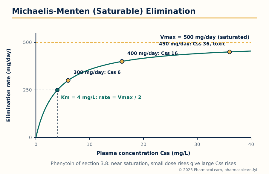 Figure: Saturable elimination in one curve. Well below Km the process is effectively first order; well above Km it is zero order at Vmax; near Km, where phenytoin is dosed, small changes have large effects.
Saturable elimination is described by the Michaelis-Menten equation, borrowed from enzyme kinetics. The rate is:
Rate of elimination = -dC/dt = (Vmax x C) / (Km + C)
where Vmax is the maximum rate of elimination when the enzymes are saturated and Km, the Michaelis constant, is the concentration at which the rate is half of Vmax. Read the equation at its limits: when C is much less than Km, the rate is approximately (Vmax / Km) x C, first order with an effective rate constant Vmax / Km; when C is much greater than Km, the rate is approximately Vmax, zero order; in between, the kinetics are mixed order, which is where therapeutic concentrations of phenytoin sit.
At steady state during regular dosing, the dosing rate R equals the elimination rate, so R = Vmax x Css / (Km + Css), which rearranges to:
Css = (Km x R) / (Vmax - R)
Worked example, phenytoin. Take Vmax = 500 mg/day and Km = 4 mg/L (values typical of an adult patient). At a dosing rate of 300 mg/day, Css = (4 x 300) / (500 - 300) = 1200 / 200 = 6 mg/L. Raise the dose to 400 mg/day: Css = (4 x 400) / (500 - 400) = 1600 / 100 = 16 mg/L. Raise it to 450 mg/day: Css = (4 x 450) / (500 - 450) = 1800 / 50 = 36 mg/L, well into the toxic range. A 33 percent dose increase (300 to 400) nearly trebled the concentration, and a further 12.5 percent increase (400 to 450) more than doubled it again. As R approaches Vmax the denominator approaches zero and Css climbs without limit: no steady state exists at or above Vmax, and the drug accumulates indefinitely. This is why phenytoin is dosed in small increments (25 to 30 mg) near target levels, with plasma level monitoring.
Estimating Km and Vmax for a patient. Measure the steady state concentrations at two different dosing rates, R1 with Css1 and R2 with Css2. Rearranging the steady state equation gives 1/R = (Km / Vmax) x (1/Css) + 1/Vmax, so a plot of 1/R against 1/Css is a straight line with intercept 1/Vmax and slope Km/Vmax: from two patient points the line, and hence both parameters, can be calculated, and the dosing rate for any target Css follows. Direct and Ludden plots are alternative graphical forms of the same algebra. Two points are a minimum, and predictions are checked against the next measured level.
3.9 Drug interactions: introduction and protein binding interactions
A drug interaction is a change in the effect or blood level of one drug caused by another drug (or food, or a herbal product), through pharmacokinetic mechanisms (absorption, distribution, metabolism, excretion, this section) or pharmacodynamic mechanisms (effects adding or opposing at the site of action, Unit 5). Pharmacokinetic interactions matter most when the affected drug has a narrow therapeutic index, a steep concentration response curve, or nonlinear kinetics, the phenytoin of section 3.8 being sensitive on all three counts.
Protein binding interactions. Only unbound (free) drug crosses membranes, acts, and is available for metabolism and excretion, so the free concentration is the working concentration. When two highly bound drugs compete for the same sites on albumin (or alpha 1 acid glycoprotein, which binds many basic drugs), one can displace the other and transiently raise its free concentration: the classic example is a sulfonamide or phenylbutazone displacing warfarin or tolbutamide. The rise is usually temporary, because the freed drug is also more available for clearance, and total concentration falls until the free concentration is close to its former value. It becomes clinically important when the displaced drug has a small Vd and a narrow therapeutic index, and it is a trap in interpretation: the measured total level falls while the free (active) level is unchanged, so dosing up against the total level can poison the patient.
3.10 Tissue binding interactions
Drug bound in tissues is in equilibrium with drug in plasma, and a second drug competing for tissue binding sites can shift drug back into plasma, changing both its concentration and its volume of distribution. The standard example is digoxin: quinidine displaces digoxin from binding sites in skeletal muscle (and also reduces its renal clearance), so the digoxin plasma concentration roughly doubles while the total amount in the body changes much less, so the digoxin dose must be reduced when quinidine starts.
3.11 Cytochrome P450 based drug interactions
Most oxidative drug metabolism runs through the cytochrome P450 (CYP) enzymes of liver and gut wall, isoforms with distinct substrate lists: CYP3A4 metabolises the largest share of marketed drugs, with CYP2D6, CYP2C9, CYP2C19, CYP1A2 and CYP2E1 covering most of the rest. Interactions occur by two opposite mechanisms:
- Enzyme inhibition. An inhibitor slows the metabolism of every substrate of that isoform, raising their concentrations. Inhibition begins with the first dose of the inhibitor: ketoconazole and itraconazole, macrolides such as erythromycin and clarithromycin, ritonavir, cimetidine and grapefruit juice (an intestinal CYP3A4 inhibitor) all raise the levels of CYP3A4 substrates such as simvastatin and ciclosporin. Some inhibitors act by mechanism based inactivation, destroying the enzyme, so the effect outlasts the inhibitor itself.
- Enzyme induction. An inducer increases the amount of enzyme (and often of transporters), speeding metabolism and lowering substrate concentrations over days to weeks as new enzyme is synthesised. Rifampicin is the most potent clinical inducer, with carbamazepine, phenytoin, phenobarbital and St John's wort also important; victim drugs include oral contraceptives, warfarin, ciclosporin and many antiretrovirals, whose failure through induction can mean contraceptive failure, transplant rejection or viral resistance. When the inducer is stopped, enzyme levels fall back over a similar period and doses must be re-adjusted.
3.12 Drug interactions linked to transporters
The transporters of Unit 1 section 1.2 are interaction sites in the gut, liver and kidney. P-glycoprotein in the intestinal wall limits absorption of its substrates; inhibitors (verapamil, quinidine, ritonavir, ciclosporin) raise the absorption and plasma levels of substrates such as digoxin, while inducers (rifampicin) lower them. Uptake transporters carry substrates into organs: the hepatic OATP transporters take up statins into the liver, and their inhibition by ciclosporin raises statin levels and muscle toxicity risk; renal organic anion and cation transporters (OAT, OCT) secrete drugs into urine, and competition there is the oldest transporter interaction in the subject: probenecid blocks tubular secretion of penicillin, deliberately prolonging its action, and also slows methotrexate excretion, raising its toxicity. Renal handling completes the list: drugs that change urinary pH change reabsorption of ionisable drugs by the ion trapping logic of section 1.3, and drugs reducing renal blood flow or filtration (NSAIDs in susceptible patients) reduce clearance of renally eliminated drugs such as lithium and digoxin.
One compartment kinetics at a glance
IV bolus:        C = C0 e^(-K t);  K from log plot;  Vd = Dose/C0;  CL = K x Vd
IV infusion:     Css = R / CL;  plateau in 4 to 5 half lives;  LD = Css x Vd
Extravascular:   C from (e^(-K t) - e^(-ka t));  Tmax = ln(ka/K)/(ka - K)
Two compartment: C = A e^(-alpha t) + B e^(-beta t);  terminal t1/2 = 0.693/beta
Nonlinear:       rate = Vmax x C / (Km + C);  Css = Km x R / (Vmax - R)
Unit 4: Drug Product Performance, In Vivo: Bioavailability and Bioequivalence
4.1 Drug product performance in vivo and the purpose of bioavailability studies
Unit 2 measured performance in the laboratory; this unit measures it in the body. The plasma concentration time curve after a dose of a product is its in vivo performance fingerprint: its height (Cmax) reflects the rate of absorption, its area (AUC) the extent, and its timing (Tmax) links the two. Bioavailability is the formal quantity: the rate and extent to which the active drug is absorbed from the product and becomes available in the systemic circulation. Bioavailability studies establish the absolute performance of a new drug (against an intravenous dose), compare formulations during development, prove that a changed or generic product performs like the established one (bioequivalence, the bulk of this unit), study food effects and interactions in vivo, and support modified release design.
4.2 Absolute and relative bioavailability
Absolute bioavailability (F) compares the product with an intravenous dose of the same drug, intravenous administration being by definition 100 percent available:
F = (AUC oral / Dose oral) / (AUC IV / Dose IV)
If the doses are equal, F is simply AUC oral / AUC IV. F must lie between 0 and 1; a value above 1 signals an error in the study or the assay.
Relative bioavailability compares one product or formulation with another non intravenous reference (a standard formulation, a solution, or the innovator product):
Relative BA = (AUC test / Dose test) / (AUC reference / Dose reference)
Worked example. A 100 mg tablet gives AUC = 480 mg·h/L; a 100 mg intravenous dose gives AUC = 600 mg·h/L. Absolute F = 480 / 600 = 0.80: eighty percent of the dose reached the systemic circulation, the missing fifth being incomplete absorption and first pass metabolism. A reformulated tablet giving AUC = 460 mg·h/L has relative bioavailability 460 / 480 = 0.958, or 95.8 percent of the reference. Whether 95.8 percent is close enough is decided by the bioequivalence statistics of section 4.4.
4.3 Methods for assessing bioavailability
- Plasma level studies. The standard method: serial blood samples after a single dose in healthy volunteers, assay of drug (and active metabolites where relevant), and calculation of AUC, Cmax and Tmax. AUC is measured to the last quantifiable concentration and extrapolated to infinity using the terminal rate constant, using sensitive, specific assays (usually LC-MS/MS).
- Urinary excretion studies. Used when plasma assay is difficult or the drug acts in the urinary tract: cumulative urinary excretion of unchanged drug is proportional to the amount absorbed, and the excretion rate profile reflects the absorption rate. It demands complete, timed collections and a drug excreted unchanged to a useful extent.
- Pharmacodynamic (acute response) methods. Where concentration cannot be measured, a quantifiable effect (blood pressure, blood glucose, pupil size) can stand in if precisely measured and related to concentration; inherently noisier, and a last resort.
- In vitro methods as surrogates. Dissolution (Unit 2) does not measure bioavailability, but with a validated IVIVC or under a BCS biowaiver (section 4.8) it can replace the in vivo study for defined cases.
Single dose studies in healthy volunteers are the norm, being the most sensitive design for detecting formulation differences; patient and multiple dose studies enter where safety or ethics require them.
4.4 Bioequivalence: the concept and the statistical rule
Two products are bioequivalent when the rate and extent of absorption of the active ingredient from them are not significantly different, so that they can be expected to be therapeutically equivalent and interchangeable. The comparison is made on log transformed AUC (extent) and Cmax (rate), because pharmacokinetic data are log normally distributed and the analysis works on ratios. The decision rule used by regulators worldwide is:
The 90 percent confidence interval for the ratio of the geometric means (test / reference) of AUC and of Cmax must lie entirely within 0.80 to 1.25 (that is, 80.00 to 125.00 percent).
The interval is asymmetric on the ordinary scale because it is symmetric on the log scale (log 0.80 = minus log 1.25), which is why the famous limits are 80 and 125 rather than 80 and 120. Two features deserve emphasis. First, it is the whole confidence interval that must fit inside the limits, not the point estimate: a study with a perfect mean ratio of 1.00 but wide variability can fail, so the study must be powered adequately, in practice enough subjects for the drug's within subject variability (commonly 12 to 36, more for highly variable drugs). Second, Tmax is usually compared descriptively, because it is a discrete sampled quantity. Narrow therapeutic index drugs are held to tighter limits by several regulators, and highly variable drugs may use widened Cmax limits under defined conditions; the 80 to 125 percent rule on log transformed data remains the reference standard used in section 4.6.
4.5 Design and evaluation of bioequivalence studies
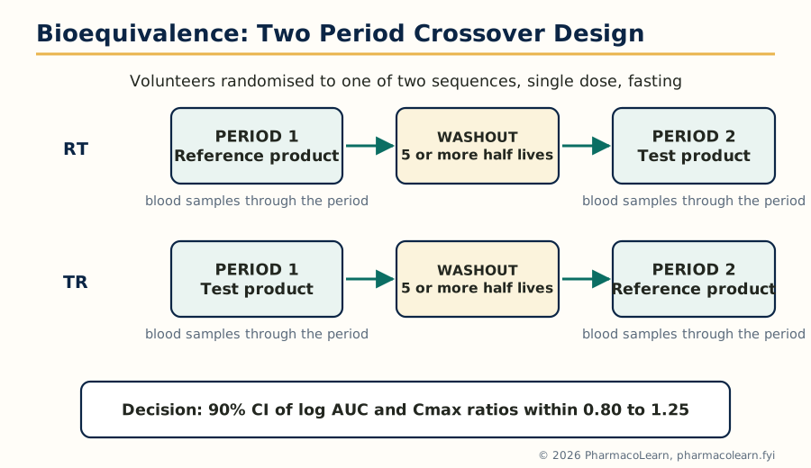 Figure: The standard 2 x 2 crossover. Each volunteer receives both products in randomised order, so each subject is their own control and the comparison is made within subjects, which is what gives the design its power.
The standard design is the single dose, two period, two sequence crossover in healthy volunteers under fasting conditions. Volunteers are randomised to sequence RT (reference, then test) or sequence TR (the reverse). The periods are separated by a washout of at least five half lives, so no drug carries over. Blood samples are taken on a schedule dense around Tmax and long enough to characterise AUC (sampled AUC should cover at least 80 percent of the extrapolated total). The crossover is chosen because within subject variability is much smaller than between subject variability, so far fewer subjects are needed than in a parallel design; its analysis (ANOVA on log transformed data) separates formulation, period, sequence and subject effects. Other designs have defined places: parallel designs for drugs with very long half lives; replicate designs (each product given twice) for highly variable drugs, which measure the reference's own within subject variability and support scaled acceptance limits; fed studies alongside fasting ones where food affects the product or labelling recommends dosing with food; and multiple dose studies where single dose data cannot represent use, now uncommon. Standardisation is part of the design: fasting state, water volume, posture, activity, diet and sampling times are all fixed by protocol, so the study exposes formulation differences, not lifestyle differences.
4.6 A bioequivalence example, evaluated
Worked example. A 24 volunteer fasting crossover study compares a generic tablet (test) with the innovator tablet (reference), 100 mg. Log transformed analysis gives: AUC geometric mean ratio = 1.02, 90 percent confidence interval 0.95 to 1.10; Cmax ratio = 0.98, interval 0.92 to 1.08; median Tmax 2.0 hours for both.
Judgement: the AUC interval (0.95 to 1.10) lies entirely within 0.80 to 1.25, and so does the Cmax interval (0.92 to 1.08); Tmax is the same. The products are bioequivalent and the generic may be approved as substitutable. Contrast the near miss: had the Cmax interval been 0.78 to 1.05, the study would fail on Cmax even though the point estimate (about 0.90) looks acceptable, because the lower bound falls outside 0.80. The interval, not the average, carries the decision.
4.7 Study submission and the drug review process
A bioequivalence study is a regulated document, not just an experiment. The sponsor submits the full study report (protocol and ethics approval, clinical and analytical reports, individual subject data, the statistical analysis, and certificates for the test and reference products including batch numbers, potency and dissolution profiles) within the marketing application, in India to the Central Drugs Standard Control Organisation (CDSCO) under the Drugs and Cosmetics Act and the New Drugs and Clinical Trials Rules, and elsewhere within an abbreviated application relying on the innovator's data. Reviewers check the design against the guideline (subjects, washout, sampling, assay validation, handling of dropouts and outliers), may audit the clinical and bioanalytical sites, and can require the raw data. Approval of the application is approval of the study: the generic is licensed as bioequivalent; section 4.8 defines the cases where the study itself may be omitted.
4.8 The biopharmaceutics classification system (BCS)
The BCS classifies drugs by aqueous solubility and intestinal permeability, each high or low against defined criteria (highly soluble: highest dose dissolves in 250 mL or less across the physiological pH range; highly permeable: absorption of 85 percent or more). The four classes:
| Class | Solubility | Permeability | Behaviour and examples |
|---|---|---|---|
| I | High | High | Rapid, complete absorption; gastric emptying often rate limiting. Examples: propranolol, metoprolol, paracetamol |
| II | Low | High | Dissolution rate limiting; bioavailability improved by particle size reduction, solubilisation. Examples: carbamazepine, glibenclamide, ketoconazole |
| III | High | Low | Permeation rate limiting; absorption variable, transporter sensitive. Examples: atenolol, cimetidine, metformin |
| IV | Low | Low | Both steps limiting; poor and variable bioavailability. Examples: furosemide, hydrochlorothiazide |
The regulatory application is the biowaiver: for immediate release products of class I drugs (and, under current harmonised guidance, defined class III cases) dissolving very rapidly, an in vivo bioequivalence study may be waived on dissolution data, because the dosage form cannot plausibly change absorption controlled by gastric emptying. Methods behind the classification are the solubility determination across pH and the permeability determination of section 4.9.
4.9 Permeability: in vitro, in situ and in vivo methods
- In vitro methods. Cell monolayers grown on filter inserts: Caco-2 cells (human colon carcinoma cells differentiating into enterocyte like cells with transporters and tight junctions) are the standard, giving apparent permeability in both directions, whose ratio exposes efflux. PAMPA (parallel artificial membrane permeability assay) measures passive permeability only, through a lipid impregnated filter, at high throughput. Excised intestinal tissue in diffusion (Ussing) chambers keeps the tissue architecture intact.
- In situ methods. The single pass intestinal perfusion in anaesthetised animals perfuses a defined intestinal segment at a known rate and calculates effective permeability from the disappearance rate, with blood supply and nerves intact. The closed loop variant injects drug into a tied off segment and measures what remains.
- In vivo methods. Human absorption is estimated from absolute bioavailability corrected for first pass, from urinary recovery, from radiolabel mass balance studies, or from marker compounds: metoprolol is the classic high permeability reference, atenolol or mannitol the low permeability references.
4.10 Generic biologics: biosimilar drug products
A biological drug (a protein made by living cells, Unit 5) cannot be copied exactly: the manufacturing process defines the product, and a second manufacturer's version will differ in detail however carefully made. Such follow on products are called biosimilars, not generics, and are not shown bioequivalent by the plasma curve method of this unit, because blood levels of a protein do not capture its structure or immunogenicity. Approval instead rests on a stepwise comparability exercise: analytical and structural comparison with the reference biologic, functional assays, comparative pharmacokinetic and pharmacodynamic studies where a marker exists, a comparative clinical study in a sensitive indication, and immunogenicity assessment, the totality of evidence substituting for identity.
4.11 Clinical significance, special concerns and generic substitution
Bioequivalence is a statistical statement about average behaviour in a study population, and its clinical use needs qualifications. Clinical significance: an approved bioequivalent generic can be substituted for the innovator with confidence for the great majority of drugs, because the 80 to 125 percent interval, on top of manufacturing controls, keeps exposure differences within the variation patients already experience between doses, days and meals. Special concerns arise for narrow therapeutic index drugs (warfarin, phenytoin, ciclosporin, levothyroxine), where small exposure changes matter and regulators apply tighter limits and clinicians monitor levels after a switch; for modified release products, whose profiles must match at several points, not only in AUC and Cmax; for drugs with nonlinear kinetics, where equivalence at one dose does not automatically prove it at another; and for patient factors (age, disease, interacting medicines) no volunteer study reproduces. Generic substitution, dispensing an approved generic in place of the prescribed brand, is the everyday consequence of the system: it lowers cost and widens access, and its safety rests on the study, the statistics, the review and manufacturing quality. Substitution between two different generics, each proven against the innovator but not against each other, is acceptable in the same framework because both are anchored to the same reference; repeated switching for narrow index drugs is nevertheless discouraged.
Unit 5: Application of Pharmacokinetics
5.1 Application to modified release drug products
Modified release products (sustained, controlled, extended release) are designed backwards from pharmacokinetics. The target is a plasma profile: a chosen concentration band held for a chosen time after a single dose, replacing several immediate release doses. The design calculation uses Unit 3 directly: the zero order input rate needed to hold a target concentration is R = target C x CL (the infusion equation of section 3.4 worn by a tablet), the immediate release loading portion is sized from the target concentration and Vd like a loading dose, and the total dose is the loading portion plus the rate multiplied by the intended duration. Pharmacokinetics also judges the result: the product shows a flattened curve (lower Cmax, later Tmax, smaller peak to trough fluctuation), its AUC must match the intended total exposure, and its in vitro release profile is tied to the plasma profile by the Level A IVIVC of section 2.9, which lets release specifications stand in for clinical performance. Two failure modes are pharmacokinetic: dose dumping, in which the entire dose releases at once (a particular danger with alcohol for some products), converting the regimen into an overdose bolus; and incomplete release, in which the tail of the dose is never released before the product leaves the gut's absorbing region.
5.2 Application to targeted drug delivery systems
Targeted delivery (MPH201T) is applied pharmacokinetics at the level of distribution. A carrier changes the drug's apparent volume of distribution and clearance routes: a liposome or nanoparticle too large for normal capillaries circulates with the plasma volume as its initial space, is cleared by the reticuloendothelial system rather than the kidney, and releases its drug on a schedule set by the carrier, so the plasma curve reflects the carrier's kinetics more than the molecule's. Evaluation therefore measures two concentrations, total drug and released (free) drug, because only the released drug acts and only it can be compared with the conventional product. A targeted product can show a much larger AUC of total drug yet deliver similar or smaller free drug exposure to most tissues, which is precisely its therapeutic point: exposure is redistributed, raised at the target (tumour, infection site) and lowered at the dose limiting organ (for liposomal doxorubicin, the heart).
5.3 Introduction to pharmacokinetics and pharmacodynamics (PK/PD)
Pharmacokinetics says what concentration the dose produces; pharmacodynamics says what effect that concentration produces; therapy needs the two joined. The link is the concentration effect relationship, typically a saturable curve described by the Emax model: Effect = (Emax x C) / (EC50 + C), where Emax is the maximum achievable effect and EC50 the concentration producing half of it. Joining the models explains everyday observations: effect lags plasma concentration when the drug must distribute to an effect site or act indirectly (the hysteresis loop when effect is plotted against concentration); effect persists after the drug leaves the plasma when binding is irreversible or the response long lived (aspirin on platelets, proton pump inhibitors); and tolerance is a time dependent change on the PD side. Antibiotic dosing is the most quantified PK/PD example: the indices predicting cure are Cmax/MIC, AUC/MIC and the time above the MIC, each matched to a class of antibiotic.
5.4 Drug interactions as an applied problem
Unit 3 sections 3.9 to 3.12 gave the mechanisms. In practice, interactions are managed by prediction (knowing the isoforms and transporters a drug uses), by design (interaction studies are part of development, and the label states doses to use with strong inhibitors and inducers), and by monitoring (levels and endpoints after any change in a narrow index patient's medicines). Interactions are pharmacokinetics in reverse: the same equations predict how much an inhibitor raises a Css (new Css = old Css x (old CL / new CL)) and how long induction takes to develop and wear off (enzyme turnover, days to weeks, not the inducer's half life).
5.5 Pharmacokinetics of biotechnology drugs: general principles
Biotechnology drugs (therapeutic proteins, monoclonal antibodies, oligonucleotides, and the products of sections 5.6 to 5.9) obey the same ADME words but by different machinery. Absorption: proteins are digested if swallowed, so they are injected; after subcutaneous injection, large molecules enter mainly through the lymphatics, slowly, so Tmax is measured in days and bioavailability is incomplete and variable. Distribution: proteins are largely confined to plasma and extracellular fluid (small Vd) and cross membranes poorly. Elimination: there is no CYP metabolism; proteins are cleared by proteolysis throughout the body, by receptor mediated endocytosis after binding their target (target mediated drug disposition, saturable, making kinetics nonlinear at low doses), by the reticuloendothelial system for particles and complexes, and, for small proteins and peptides below the filtration size, by the kidney. Immunogenicity overlays everything: anti drug antibodies can accelerate clearance, neutralise activity, or both, and can appear or grow during treatment, so biotechnology kinetics is partly a moving target in a way small molecule kinetics is not.
5.6 Proteins and peptides
Therapeutic proteins and peptides divide by size and origin: replacement proteins (insulin, growth hormone, erythropoietin, clotting factors), enzymes, cytokines and peptide hormones. Their behaviour follows section 5.5 with peptide specific features: small peptides are filtered by the kidney and attacked by peptidases, so natural peptides often have half lives of minutes, and medicinal chemistry buys time: sequence changes resisting peptidases, and above all PEGylation (covalent attachment of polyethylene glycol), which enlarges the molecule beyond the filtration size, shields it from proteases and antibodies, and can stretch a half life from hours to days, as in pegfilgrastim and peginterferon. Insulin is the model system: its formulations (rapid, short, intermediate and long acting) engineer the absorption rate from the injection site to sculpt the plasma profile, the extravascular mathematics of section 3.5 in therapeutic use.
5.7 Monoclonal antibodies
Monoclonal antibodies (immunoglobulin G molecules engineered against a single target: trastuzumab against HER2, rituximab against CD20, adalimumab against TNF) are the largest class of biotechnology drugs. Their pharmacokinetics is distinctive: given intravenously or subcutaneously (bioavailability typically 50 to 80 percent subcutaneously, absorbed through the lymph over several days); distributed in a volume close to plasma plus accessible interstitial fluid; eliminated by proteolysis after cellular uptake, with target mediated clearance adding a saturable component, large when target is abundant and dose small, so clearance falls as dose rises until that pathway saturates; and recycled by FcRn, giving half lives of typically 2 to 4 weeks. Elimination is neither renal nor CYP based, so organ impairment and classic CYP interactions matter far less than for small molecules. Anti drug antibodies, when they form, can clear the antibody rapidly and destroy the response.
5.8 Oligonucleotides
Oligonucleotide drugs (antisense oligonucleotides and small interfering RNAs, and related aptamers of MPH201T) are short synthetic nucleic acid chains that bind a target RNA and change the protein made from it. Their pharmacokinetics is a chemistry story: unmodified oligonucleotides are destroyed by nucleases in minutes, so marketed molecules carry stabilising chemistry (phosphorothioate backbones, 2 prime sugar modifications) that also makes them bind plasma proteins, keeping them in circulation and delivering them to tissues, above all liver and kidney. Plasma half life is short (hours) because tissue distribution is fast, but tissue half life is long (weeks), the molecule being stable inside cells and its effect lasting until the target RNA and protein turn over: dosing intervals of weeks to months follow from the tissue, not the plasma, kinetics. Delivery is the limiting problem: most tissues take up oligonucleotides poorly, solved for the liver by conjugating the molecule to a GalNAc ligand for a liver cell receptor, the strategy behind several approved siRNA drugs. Elimination is by nuclease metabolism to shorter fragments excreted in urine; CYP enzymes are not involved.
5.9 Vaccines (immunotherapy) and gene therapies
Vaccines and gene therapies stretch the pharmacokinetic framework to its limit. A vaccine is not meant to maintain a plasma concentration: its product is an immune response, so its evaluation is pharmacodynamic almost by definition: antigen dose, the adjuvant, the kinetics of antigen presentation and antibody production, and the persistence of immune memory, the therapeutic quantity, measured in years. (The PCI text lists vaccines under the heading immunotherapy.) Gene therapies deliver a nucleic acid that makes the patient's own cells produce a protein, by viral vectors (adeno associated virus above all) or by lipid nanoparticles carrying mRNA. Their disposition studies measure biodistribution and persistence of the vector and duration of expression rather than a plasma curve: a one time treatment whose expression may last years, with vector clearance, shedding in body fluids, and immune responses to the vector as the studied quantities. The conventional parameters of Unit 3 apply to the carrier and the early phase, after which pharmacology is governed by expression and cell turnover.
The subject in one chain
Dissolution (Unit 1) decides whether the drug is available to absorb
Permeation and first pass decide the fraction that survives (Units 1, 4)
Compartment kinetics turn the curve into parameters (Unit 3)
Bioequivalence proves a new product matches the old (Unit 4)
PK/PD and biotechnology apply the same thinking to harder drugs (Unit 5)
Frequently Asked Questions
Q: What is the difference between biopharmaceutics and pharmacokinetics? Biopharmaceutics studies how the drug's properties, the dosage form and the body's physiology together decide how much drug becomes available and how fast. Pharmacokinetics measures and models what then happens in the body over time, expressing absorption, distribution, metabolism and excretion as parameters such as clearance, volume of distribution, half life and AUC.
Q: Why does the Noyes-Whitney equation matter to a formulator? Because it names every lever controlling dissolution rate in one expression: dM/dt = (D x A / h) x (Cs - C). Increasing surface area A by micronisation, raising Cs by salt or solid form selection, and reducing diffusion layer thickness h by agitation each raise the rate proportionally. For a poorly soluble, dissolution limited drug, these are the main tools for improving bioavailability.
Q: What is the pH-partition theory, and what is its main limitation? The theory states that membranes are crossed mainly by the unionised fraction, so a weak acid is best absorbed where it is unionised (acidic fluid) and a weak base where it is unionised (alkaline fluid), the proportions coming from the Henderson-Hasselbalch equation. Its main limitation is that it ignores surface area and blood flow: weak acids are in practice absorbed mainly from the small intestine, not the stomach, because the intestine offers an enormous surface.
Q: How are K, half life, Vd, clearance and AUC obtained from an IV bolus study? Plot log plasma concentration against time; the straight line's slope gives K (slope = minus K / 2.303) and its intercept gives C0. Then t1/2 = 0.693 / K, Vd = Dose / C0, AUC = C0 / K, and CL = K x Vd, which must agree with Dose / AUC.
Q: Why does steady state take 4 to 5 half lives, and what decides the steady state level? During constant infusion or repeated dosing, drug accumulates because each interval adds drug while elimination removes a fraction of what is present; concentration approaches its plateau exponentially with the elimination rate constant, reaching about 90 percent in 3.32 half lives and practical steady state in 4 to 5 half lives, whatever the dose. The level itself is set by input and clearance alone: Css = infusion rate / CL (or F x Dose / (CL x interval) orally). Changing the dose changes the level, not the time to reach it.
Q: What is the flip-flop phenomenon? After extravascular dosing, the terminal slope of the log concentration curve reflects the slower of absorption (ka) and elimination (K). Normally ka is larger and the slope gives K; if absorption is slower than elimination, as with many sustained release products, the slope gives ka instead. Reading it as K misreports the absorption half life as the elimination half life: this reversal is flip-flop kinetics, suspected whenever a modified release product appears to have a much longer half life than the same drug given intravenously.
Q: Why is phenytoin the classic example of nonlinear pharmacokinetics? Phenytoin is eliminated by a saturable (Michaelis-Menten) pathway, and therapeutic concentrations sit near Km, in the mixed order region. Its steady state concentration is Css = Km x R / (Vmax - R), so as the dosing rate R approaches Vmax, Css rises disproportionately: with Vmax 500 mg/day and Km 4 mg/L, raising the dose from 300 to 400 mg/day raises Css from 6 to 16 mg/L, and 450 mg/day gives a toxic 36 mg/L. Small dose increments and level monitoring are therefore mandatory.
Q: What are the acceptance limits for bioequivalence, and why 80 to 125 percent? The 90 percent confidence interval for the ratio of geometric means (test over reference) of log transformed AUC and Cmax must lie entirely within 0.80 to 1.25. The limits are symmetric on the log scale (log 0.80 = minus log 1.25), which is why the upper limit is 125 and not 120. It is the whole interval, not the mean ratio, that must fit, so an imprecise study can fail even with a mean ratio near 1.00.
Q: What is the biopharmaceutics classification system and what is a biowaiver? The BCS classifies drugs by solubility and permeability into four classes: I high/high, II low/high, III high/low, IV low/low, and so predicts which step limits absorption (dissolution for class II, permeation for class III). A biowaiver waives the in vivo bioequivalence study for an immediate release class I product (and defined class III cases) dissolving very rapidly, accepting dissolution data instead, because absorption of such a drug is controlled by gastric emptying and cannot plausibly differ between fast dissolving products.
Q: Why can a biosimilar not be approved by an ordinary bioequivalence study? A biosimilar is a protein made by a different living cell process, so it is highly similar to the reference biologic but never structurally identical. Plasma curves cannot prove two such molecules share structure, potency and immunogenicity, so approval rests on a stepwise comparability exercise: analytical and functional comparison, comparative pharmacokinetic and pharmacodynamic data where a marker exists, clinical comparison in a sensitive population, and immunogenicity testing, judged as a totality of evidence.
Complete MPH202T notes, all 5 units in one PDF, free to keep.
Other M.Pharm subjects: MPH101T · MPC101T · MPL101T · MPH102T · MPH103T · MPH104T · MPL102T · MPL103T · MPL104T · MPC102T · MPC103T · MPC104T · MPH201T · MPH202T · MPH203T · MPH204T · MPC201T · MPC202T · MPC203T · MPC204T · M.Pharm