
MPC203T — Computer Aided Drug Design
4 hrs/week, 4 credits, 60 hours, 100 marks (75 end semester + 25 sessional). Notes follow the M.Pharm syllabus, unit by unit.
MPC203T Computer Aided Drug Design notes for M.Pharm Semester 2 Pharmaceutical Chemistry: CADD history, QSAR parameters, Hansch and Free Wilson analysis, 3D QSAR, molecular modeling and docking, ADMET prediction, de novo design and virtual screening, free unit wise PDF downloads on PharmacoLearn.
Units in this subject
- Unit 1 — Introduction to Computer Aided Drug Design (CADD): history, different techniques and applications; Quantitative Structure Activity Relationships: basics, history and development of QSAR; physicochemical parameters and methods to calculate physicochemical parameters: Hammett equation and electronic parameters (sigma), lipophilicity effects and parameters (log P, pi substituent constant), steric effects (Taft steric and MR parameters); experimental and theoretical approaches for the determination of these physicochemical parameters
- Unit 2 — Quantitative Structure Activity Relationships: Applications: Hansch analysis, Free Wilson analysis and relationship between them, advantages and disadvantages; deriving 2D-QSAR equations; 3D-QSAR approaches and contour map analysis; statistical methods used in QSAR analysis and importance of statistical parameters
- Unit 3 — Molecular Modeling and Docking: molecular and quantum mechanics in drug design; energy minimization methods: comparison between global minimum conformation and bioactive conformation; molecular docking and drug receptor interactions: rigid docking, flexible docking and extra precision docking; agents acting on enzymes such as DHFR, HMG-CoA reductase and HIV protease, cholinesterase (AChE and BChE)
- Unit 4 — Molecular Properties and Drug Design: prediction and analysis of ADMET properties of new molecules and its importance in drug design; de novo drug design: receptor/enzyme interaction and its analysis, receptor/enzyme cavity size prediction, predicting the functional components of cavities, fragment based drug design; homology modeling and generation of 3D structure of protein
- Unit 5 — Pharmacophore Mapping and Virtual Screening: concept of pharmacophore, pharmacophore mapping, identification of pharmacophore features and pharmacophore modeling; conformational search used in pharmacophore mapping; in silico drug design and virtual screening techniques: similarity based methods and pharmacophore based screening, structure based in silico virtual screening protocols
Download MPC203T PDF Notes
Free PDFs for this subject, one per unit:
Computer Aided Drug Design, subject code MPC203T, is a core Semester 2 subject of M.Pharm Pharmaceutical Chemistry. It carries 4 credits and 60 hours of theory, taught at 4 hours per week, for 100 marks.
This subject teaches how computers are used to design drug molecules before, and sometimes instead of, making them in the laboratory. Unit 1 introduces computer aided drug design (CADD) and the foundations of quantitative structure activity relationships (QSAR): the physicochemical parameters, electronic, lipophilic and steric, that connect a structure to its activity. Unit 2 applies those parameters in Hansch analysis and Free Wilson analysis, shows how 2D QSAR equations are derived, moves to 3D QSAR and contour maps, and covers the statistical methods that decide whether a model is real or a mirage. Unit 3 is molecular modeling and docking: molecular and quantum mechanics, energy minimization, the difference between the global minimum and the bioactive conformation, and docking into the enzyme targets the syllabus names, DHFR, HMG CoA reductase, HIV protease and the cholinesterases. Unit 4 turns to molecular properties: prediction of ADMET behaviour, de novo and fragment based design, and homology modeling of proteins whose structures are unknown. Unit 5 finishes with pharmacophore mapping and virtual screening, the techniques that search whole databases for the next lead. A student who completes this subject should be able to read a QSAR equation and judge it, explain what a docking program actually does, and plan a sensible in silico screening protocol.
Unit 1: Introduction to Computer Aided Drug Design and QSAR Basics
1.1 Why drug design needed computers
A modern drug discovery programme tests chemistry against biology at industrial scale, and it is slow and expensive: a new medicine typically takes well over a decade to reach patients, and most candidate molecules fail along the way, usually because they are not absorbed, are metabolised too fast, or turn out to be toxic. Synthesis is the bottleneck of classical medicinal chemistry. Every analogue in a series costs days of bench work, and a chemist can only explore the ideas that can physically be made and assayed. Computer aided drug design attacks that bottleneck by moving part of the exploration into the computer. A model can estimate the activity of a compound that does not exist yet, a docking program can test whether a proposed molecule fits its target before a flask is charged, and a screening protocol can search millions of structures overnight and hand the chemist a shortlist worth making. CADD does not replace experiment; it decides which experiments are worth doing. Two broad strategies run through the whole subject. Ligand based design works from known active molecules and infers the features activity requires, the home ground of QSAR and pharmacophore methods. Structure based design works from the three dimensional structure of the target protein and designs molecules to fit it, the home ground of docking, de novo design and homology modeling. Most real projects use both, and this course teaches them in that order.
1.2 The CADD toolbox: techniques and applications
Target discovery and validation
        |
        v
Hit identification ---- virtual screening, docking, HTS support
        |
        v
Hit to lead ----------- QSAR, pharmacophore models, similarity search
        |
        v
Lead optimisation ----- Hansch analysis, 3D QSAR, ADMET prediction
        |
        v
Candidate selection --- free energy estimates, selectivity models
        |
        v
Synthesis and biological testing (the computer advises, the lab decides)
The main techniques, each developed in later units, are:
- QSAR: mathematical equations linking activity to measurable or calculable properties of a series, used to predict the next analogues to make (Units 1 and 2).
- Molecular modeling: building and manipulating molecular structures in three dimensions, minimising their energy and exploring their shapes (Unit 3).
- Molecular docking: placing a ligand into the binding site of a target and scoring the fit, used for screening and for understanding binding (Unit 3).
- ADMET prediction: in silico estimates of absorption, distribution, metabolism, excretion and toxicity, used to kill weak candidates early (Unit 4).
- De novo and fragment based design: constructing new molecules inside a binding site, or growing them from small binding fragments (Unit 4).
- Homology modeling: building a model of a protein whose experimental structure is unknown, from the structure of a relative (Unit 4).
- Pharmacophore mapping and virtual screening: abstracting the essential features of active molecules and using them, or docking, to search large databases (Unit 5).
Applications follow from the list: prioritising compounds for synthesis, explaining why a series behaves as it does, finding new chemotypes for a known target, flagging ADMET liabilities before animal work, and rescuing projects where no crystal structure exists. The honest limitation belongs in the same breath: a model is only as good as the data and assumptions inside it, and every in silico prediction of consequence is eventually checked at the bench.
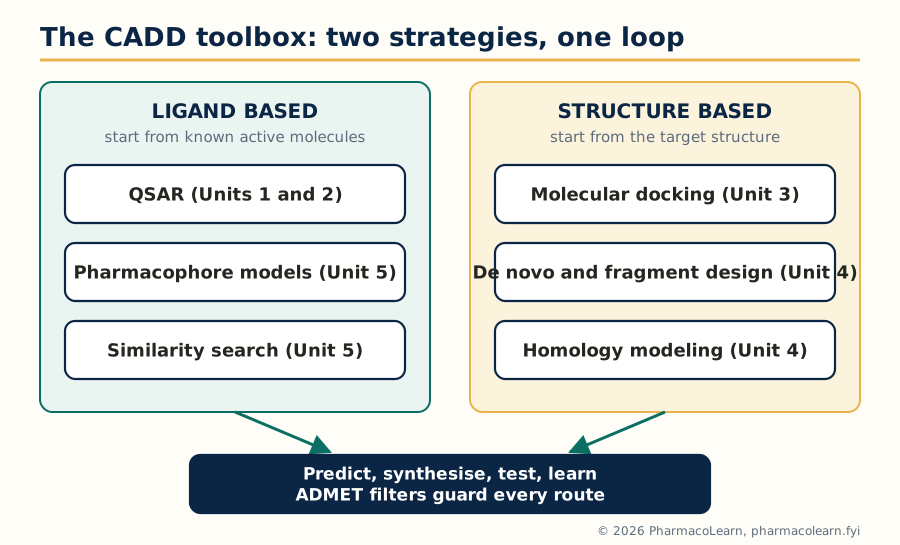
Figure: Ligand based methods learn from known actives, structure based methods from the target; both feed the same predict, synthesise and test loop, with ADMET filters on guard.
1.3 A short history of the subject
The idea that structure determines activity is older than the computer by a century. In 1868 Crum Brown and Fraser proposed that the physiological action of a compound is a function of its chemical constitution, the founding statement of structure activity thinking. Around 1900 Meyer and Overton independently linked narcotic potency to oil water partitioning, the first lipophilicity relationship. Hammett, in the 1930s, gave physical organic chemistry its sigma rho equation for electronic effects in benzene derivatives, the direct ancestor of QSAR parameters. The quantitative era opened in the early 1960s: Hansch and co workers combined lipophilic, electronic and steric parameters in multiple regression equations (the Hansch approach, 1962 to 1964), and Free and Wilson published their additive group contribution model in 1964. Through the 1970s and 1980s, molecular graphics and force fields made molecules visible and manipulable on screen, the first docking programs appeared, and in 1988 Cramer introduced CoMFA, the first practical 3D QSAR method. The 1990s added combinatorial libraries, high throughput screening and Lipinski's rule of five (1997), which defined the property space of oral drugs. The modern era runs on thousands of experimental protein structures, cheap computing, and machine learning methods layered on the classical ones. The exam relevant point is the logic of the history: each generation of technique answers the weakness of the one before, and the classical methods in this syllabus are still the interpretive core of the newer ones.
1.4 SAR versus QSAR: the basic idea
A structure activity relationship (SAR) is a qualitative account: in this series, a chloro substituent raises activity, a hydroxyl lowers it, moving the side chain kills it. SAR is read from tables of analogues and guides intuition. A quantitative structure activity relationship (QSAR) goes one step further and makes the relationship mathematical: the biological activity of a series of compounds is expressed as an equation in terms of their physicochemical properties or structural descriptors, for example log (1/C) equals some combination of log P, sigma and a steric term plus a constant. Three consequences follow. First, the equation can predict the activity of compounds not yet synthesised, which is the economic point of the exercise. Second, the coefficients are interpretable: a positive coefficient on log P says activity rises with lipophilicity in this series, a negative one on sigma says electron donating groups help, and so on. Third, the model can be tested statistically, and Unit 2 insists on that testing. Activity in QSAR is almost always handled in logarithmic form, log (1/C), where C is the molar concentration producing a standard effect (an IC50, EC50 or minimum effective dose), because free energy of binding is proportional to the logarithm of an equilibrium or potency term: equal steps in log activity correspond to equal steps in binding free energy, which is what substituent effects actually add up to.
1.5 Physicochemical parameters: the three families
QSAR parameters fall into three families, and the syllabus names a champion for each.
| Family | What it captures | Syllabus parameters |
|---|---|---|
| Electronic | The electron pushing or pulling effect of a substituent on reaction centres and binding interactions | Hammett sigma constants, derived from ionisation of benzoic acids |
| Lipophilic | The tendency of a molecule or substituent to leave water for a fatty phase, governing transport and hydrophobic binding | log P of the whole molecule, pi substituent constant |
| Steric | The size and bulk of a substituent, governing fit into a pocket and access to a centre | Taft Es constant, molar refractivity (MR) |
A fourth, informal group completes the working set: structural and indicator parameters, such as counts of hydrogen bond donors and acceptors, molecular weight, and indicator variables that simply record the presence (1) or absence (0) of a feature. The art of QSAR is choosing a small set of parameters that are not strongly intercorrelated, because two parameters carrying the same information destabilise the regression and confuse the interpretation.
1.6 Electronic parameters: the Hammett equation and sigma
Hammett studied the ionisation of substituted benzoic acids in water and defined the substituent constant sigma by comparing each substituted acid with benzoic acid itself: sigma equals log (K_X divided by K_H), where K_X is the ionisation constant of the substituted acid and K_H that of the parent. A substituent that withdraws electrons stabilises the carboxylate anion, increases ionisation and earns a positive sigma; an electron donating substituent earns a negative one. Illustrative textbook values: para nitro, sigma about plus 0.78 (strongly withdrawing); para chloro, about plus 0.23; hydrogen, zero by definition; para methyl, about minus 0.17; para methoxy, about minus 0.27 (donating by resonance). Meta and para positions have separate constants (sigma_m and sigma_p) because resonance donation reaches the para position but not the meta. The Hammett equation generalises the idea to any reaction or equilibrium influenced by the same substituents: log (k_X divided by k_H) equals rho multiplied by sigma. The reaction constant rho measures how sensitive that particular reaction is to electronic effects; rho near 1 by construction for the benzoic acid ionisation itself, positive rho means the process is helped by electron withdrawal, negative rho that it is helped by donation. A worked micro example: for a reaction series with rho equal to 1.00, a para nitro group changes log (k/k0) by 1.00 times 0.78, that is 0.78 log units, roughly a sixfold rate increase. In drug series the same logic applies to binding: if activity correlates with sigma with a positive coefficient, electron withdrawing substituents favour activity, a mechanistic clue about the interaction in the binding site.
1.7 Lipophilicity: log P, log D and the pi constant
Lipophilicity is the single most used parameter in drug design, because a drug must dissolve in water well enough to be carried, yet cross fatty membranes well enough to reach its target, and then often bind a hydrophobic pocket. It is measured by the partition coefficient P, the ratio of the concentration of the unionised compound in n octanol to its concentration in water at equilibrium, and quoted as log P. n Octanol is the standard organic phase because its hydroxyl head and hydrocarbon tail make it a crude but serviceable model of a membrane. Two refinements matter. log D, the distribution coefficient, counts all species, ionised and unionised, at a stated pH (usually 7.4), and is the relevant number for ionisable drugs in the body. The pi substituent constant (Hansch and Fujita) isolates one substituent's contribution: pi_X equals log P of the substituted parent minus log P of the unsubstituted parent. Worked example: log P of benzene is 2.13 and of toluene 2.69, so pi for a methyl group is 2.69 minus 2.13, which equals 0.56; methyl adds about half a log unit of lipophilicity wherever it is attached. Pi values let a chemist price a substitution before making it, and they add: a compound's log P can be estimated by summing the parent value and the pi values of its substituents, with corrections where substituents interact.
1.8 Determining log P: experimental and theoretical approaches
The syllabus explicitly asks for experimental and theoretical approaches to the parameters, and log P is the model case.
- Shake flask method (experimental, the reference method): the compound is shaken between pre saturated octanol and water, the phases are separated, and the concentration in each is measured, usually by UV spectroscopy or HPLC. It is accurate but slow, needs pure material, and struggles with very lipophilic or very hydrophilic compounds.
- Chromatographic methods (experimental): reversed phase HPLC retention correlates with log P after calibration with standards of known value; thin layer variants exist. Faster and usable for mixtures, but indirect.
- Computational methods (theoretical): fragment based programs, of which CLOGP is the classic, add up contributions of the molecule's fragments with correction factors; atom based methods assign a contribution to every atom type; property based methods use calculated surface and charge descriptors. They are instant and need no material, but their accuracy depends on how well the fragment library covers the chemistry in hand, and unusual structures can be badly wrong.
- For sigma and the steric constants the same pattern holds: sigma comes from measured ionisation constants (experimental) or is looked up from extensive tables for new work, and calculated electronic descriptors from quantum chemistry (charges, orbital energies) increasingly serve as theoretical substitutes.
The working rule: calculated values screen thousands of ideas, measured values anchor the model where it matters.
1.9 Steric parameters: Taft Es and molar refractivity
Bulk matters when a substituent must fit a pocket or shield a centre. Taft's steric parameter Es comes from the acid catalysed hydrolysis of substituted acetates, a reaction almost insensitive to electronic effects but very sensitive to crowding near the reaction centre. Es is defined as log (k_X divided by k_H) for that hydrolysis, with methyl set to zero; bulky groups slow the reaction and earn negative values, tert butyl being around minus 1.54 on the classic scale, a quantitative statement that it is much bulkier than methyl. Molar refractivity (MR) is a whole substituent size measure derived from the refractive index and density, MR equals a function of refractive index and molar volume; it scales with the substituent's volume and polarisability, so it carries both a steric meaning (bulk) and a hint of dispersion interaction strength. MR is positive and grows with size, roughly 1.03 for hydrogen and about 5.65 for a methyl group on the usual scaled units, and Hansch equations often use MR where Es is unavailable. The two constants are not interchangeable: Es measures bulk near an attachment point, MR measures total bulk, and choosing between them is part of model building.
1.10 Indicator variables and other working parameters
Some structural facts are yes or no, and QSAR handles them with indicator variables: I equals 1 if the molecule carries an ortho substituent, a free phenolic hydroxyl, a basic nitrogen able to be protonated, a particular ring system, and 0 otherwise. Their coefficients measure the activity bonus or penalty of that feature. Alongside them sit global descriptors used throughout design: molecular weight, polar surface area, counts of hydrogen bond donors and acceptors, and the molecule's ionisation constant pKa, which decides how much of the drug is unionised and membrane permeant at intestinal and plasma pH. These descriptors return in Unit 4 as the raw material of ADMET prediction and drug likeness rules.
1.11 Unit 1 summary table
| Parameter | Symbol | What a positive value means | Typical source |
|---|---|---|---|
| Hammett constant | sigma | Substituent withdraws electrons | Ionisation of substituted benzoic acids |
| Reaction constant | rho | Process is favoured by electron withdrawal | Slope of Hammett plot |
| Partition coefficient | log P | Compound prefers octanol, lipophilic | Shake flask, HPLC, CLOGP calculation |
| Substituent lipophilicity | pi | Substituent adds lipophilicity | Difference of log P values |
| Taft constant | Es | Substituent is small near the centre (bulk gives negative) | Acid hydrolysis rates of acetates |
| Molar refractivity | MR | Substituent is large and polarisable | Refractive index and density, or tables |
With the parameters in hand, Unit 2 does the arithmetic: building equations from them, testing the equations, and reading what they say.
Unit 2: Quantitative Structure Activity Relationships: Applications
2.1 The Hansch approach: putting the parameters together
Hansch's insight was that biological activity is the product of a journey and an arrival. The molecule must first travel, through aqueous and lipid compartments in series, to the target (governed above all by lipophilicity), and must then interact with the target (governed by electronic and steric fit). The Hansch equation therefore combines the parameter families in one regression, of the general form: log (1/C) equals a coefficient times log P, plus a coefficient times sigma, plus a coefficient times a steric term, plus a constant. Each term reads like a sentence. The log P term prices transport and hydrophobic binding. The sigma term prices the electronic demands of the interaction. The steric term prices fit. The constant absorbs the activity of the parent scaffold. Because the parameters were designed to be independent, the equation can in principle separate effects that a qualitative SAR tangles together, and tell the chemist, for the next analogue, whether to raise lipophilicity, donate electrons, or cut bulk. Hansch analysis needs a congeneric series, a single scaffold with varied substituents, consistent biological data measured the same way, and enough compounds to support the number of fitted terms, the working rule being at least five compounds per parameter.
2.2 The parabolic model and optimum lipophilicity
Activity does not rise with log P forever. A very hydrophilic compound cannot cross membranes; a very lipophilic one cannot dissolve, gets trapped in the first membrane it meets, binds plasma proteins and fat, and never arrives. Hansch therefore added a squared term: log (1/C) equals minus a times (log P) squared, plus b times log P, plus the other terms and the constant. Plotted against log P at fixed other parameters, the equation is an upside down parabola with an optimum, log P0, at its peak, found by setting the derivative to zero: log P0 equals b divided by 2a. The bilinear model is a refinement often used in its place, rising linearly then falling linearly with a break near the optimum, but the parabola is the syllabus model and the teaching point stands: there is a best lipophilicity for a series acting by this mechanism, often near log P 2 for centrally acting drugs that must cross the blood brain barrier, and designing beyond the optimum in either direction wastes synthesis. A related practical tool is the Craig plot, which scatters substituents on axes of pi against sigma so the chemist can pick a test set of substituents spread across all four quadrants, varying lipophilicity and electronics independently, instead of testing ten variations of the same idea.
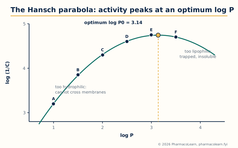
Figure: The worked example of section 2.3 plotted: activity rises with log P, peaks at the optimum log P0 of 3.14, and falls as compounds grow too lipophilic to reach the target.
2.3 Worked example: deriving a 2D QSAR equation
Consider six analogues of one scaffold with measured log P and activity log (1/C), the kind of small teaching set used to show the method (real projects use far more compounds):
| Compound | log P | Observed log (1/C) |
|---|---|---|
| A | 1.0 | 3.20 |
| B | 1.5 | 3.85 |
| C | 2.0 | 4.30 |
| D | 2.5 | 4.60 |
| E | 3.0 | 4.75 |
| F | 3.5 | 4.70 |
Step 1, fit a straight line. Least squares regression of activity on log P gives: log (1/C) equals 0.600 log P plus 2.883, with n equal to 6, r equal to 0.926, r squared equal to 0.857, s equal to 0.257 and F equal to 23.9. Step 2, look at the residuals, observed minus predicted: minus 0.283, plus 0.067, plus 0.217, plus 0.217, plus 0.067, minus 0.283. The pattern is systematic, negative at both ends and positive in the middle, the fingerprint of a curve forced into a line. Step 3, add the squared term, as section 2.2 prescribes: log (1/C) equals minus 0.336 (log P) squared plus 2.111 log P plus 1.429, with n equal to 6, r squared equal to 0.999 and s equal to 0.011; the residuals are now tiny and patternless. Step 4, read the model. The optimum is log P0 equals 2.111 divided by (2 times 0.336), which is 3.14, and the predicted peak activity is about 4.74, matching compound E, after which activity falls, exactly as compound F shows. Step 5, use and respect the model. It predicts that a new analogue at log P 3.1 should be near the peak of the series, and that money spent pushing log P to 4 would be wasted; it says nothing reliable about log P 5, outside the fitted range, because extrapolation is where QSAR models go to die. The example is deliberately small; the statistical cautions of sections 2.9 and 2.10 apply with full force.
2.4 The steps of building a QSAR model
1. Assemble the series ...... same scaffold, same assay, reliable data
        |
        v
2. Choose descriptors ....... parameters that vary and are not collinear
        |
        v
3. Fit the equation ......... multiple linear regression
        |
        v
4. Test the statistics ...... r squared, s, F, cross validated q squared
        |
        v
5. Validate ................. hold out compounds, predict, compare
        |
        v
6. Interpret and design ..... predict new analogues, synthesise, retest
Every step has a failure mode this course repeats like a refrain: mixed assays poison step 1, correlated descriptors poison step 2, too many terms poison step 3, skipped validation poisons step 5, and ignoring the model's range poisons step 6.
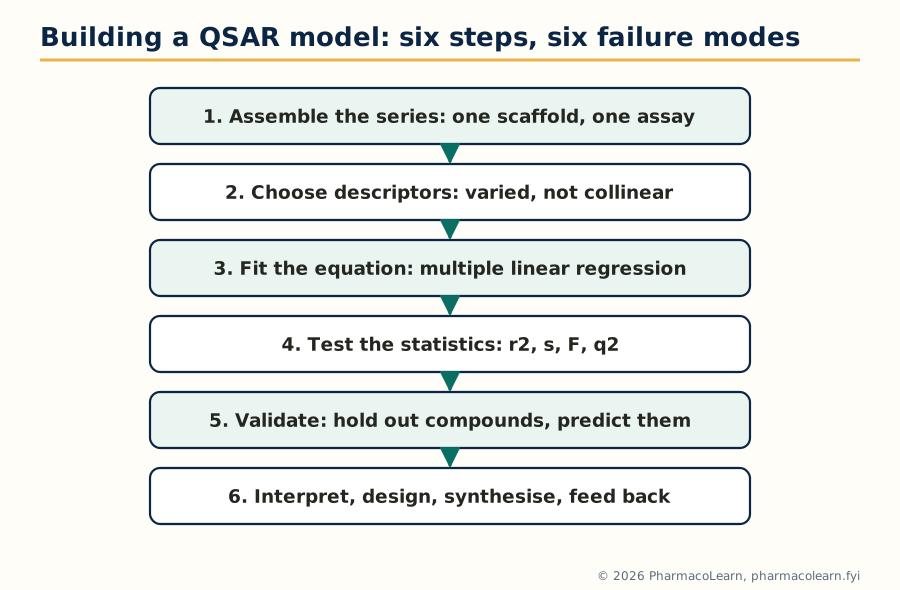
Figure: The QSAR workflow of section 2.4; the validation steps, 4 and 5, are the ones that separate a model from a mirage.
2.5 Free Wilson analysis: activity as a sum of contributions
Free and Wilson (1964) took the opposite route to Hansch. Ignore physicochemical parameters entirely; assume instead that each substituent at each position contributes a fixed amount to the activity, whatever the rest of the molecule, and that contributions add. The model is written: log (1/C) equals the sum over positions and substituents of (indicator for that substituent times its contribution) plus mu, the activity of the unsubstituted parent. Each compound is coded by a row of ones and zeros recording which substituents it carries, and regression solves for the contributions. A small worked miniature: suppose the parent of a series has log (1/C) equal to 4.00, regression assigns a chloro group at position R1 a contribution of plus 0.42, and a methoxy group at position R2 a contribution of minus 0.18. A compound carrying both is predicted at 4.00 plus 0.42 minus 0.18, that is 4.24, and a compound with chloro at R1 alone at 4.42. The output is a league table of substituents at each position, ranked, which is exactly the shopping list a chemist wants. The method's price: it can only talk about substituents it has seen, at positions it has seen, and it says nothing about why a contribution is positive. It also needs a well populated data matrix; a substituent appearing once gets a contribution fitted to a single measurement.
2.6 Hansch and Free Wilson compared, and the mixed approach
| Aspect | Hansch analysis | Free Wilson analysis |
|---|---|---|
| Basis | Physicochemical parameters (log P, sigma, steric) | Indicator variables for substituents |
| Explains mechanism | Yes, coefficients interpret transport and binding demands | No, ranks contributions without explaining them |
| Predicts new substituents | Yes, if their parameters are known | No, only substituents present in the training set |
| Data needs | Parameter values for each substituent; fewer compounds per idea | Many compounds to populate each position and substituent |
| Fails when | The series spans more than one binding mechanism | Additivity breaks down (substituents interact) |
The two are mathematically related: if substituent contributions happen to be linear functions of Hansch parameters, a Free Wilson model reduces to a Hansch model, and de novo, the founders showed the approaches are special cases of one framework. The mixed approach therefore combines them: Hansch parameters for what they can explain, plus indicator variables for structural features (a hydrogen bond donor here, a ring closure there) that parameters miss. Modern descriptor based QSAR is the mixed approach grown up: hundreds of calculated descriptors in place of the classic handful, with the same duties of validation.
2.7 3D QSAR: CoMFA and CoMSIA
2D methods never ask where in space a substituent sits. 3D QSAR does. In Comparative Molecular Field Analysis (CoMFA, Cramer 1988), the molecules of a series are first aligned in space on a common frame, a step on which everything depends. A three dimensional grid is laid around them, and at each grid point a probe atom measures two fields: the steric field (van der Waals interaction energy) and the electrostatic field (Coulomb interaction with a unit positive charge). Thousands of grid values become the descriptors, and partial least squares (PLS) regression, built to handle many correlated descriptors, fits them to activity. CoMSIA (Comparative Molecular Similarity Indices Analysis) extends the idea with smoother similarity based fields, adding hydrophobic and hydrogen bond donor and acceptor fields alongside steric and electrostatic, and is less sensitive to exactly where the grid cut offs fall. Both methods answer the question 2D QSAR cannot: not just which substituent, but where in space bulk, charge, or a hydrogen bond is wanted.
2.8 Reading contour maps
The product of a 3D QSAR run is a contour map drawn around a reference molecule. By the standard CoMFA colour convention, green contours mark regions where added steric bulk raises activity and yellow regions where bulk lowers it; blue contours mark regions where a positive charge, or an electron poor group, is favoured, and red regions where negative charge or an electron rich group is favoured. CoMSIA adds colours for hydrophobic and hydrogen bonding fields. Reading a map is the design act itself: a green contour beyond a methyl group says grow the molecule there; a yellow shell around a ring says the pocket is tight; a red contour near a carbonyl says the target wants electron density at that point in space. Contour map analysis carries two warnings. The map is only as good as the alignment, and a wrong alignment manufactures persuasive nonsense. And the map interpolates within the chemistry tested; it cannot describe a binding feature no training molecule ever probed.
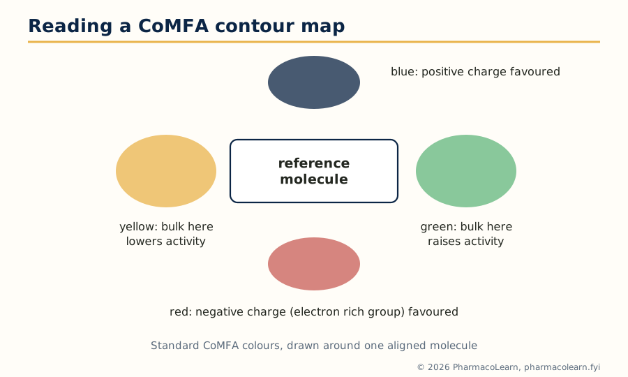
Figure: A CoMFA map in words: green wants bulk, yellow forbids it, blue wants positive charge, red wants negative charge, each in a defined region of space.
2.9 Statistical methods used in QSAR analysis
The fitting engine of classical QSAR is multiple linear regression (MLR), which finds the coefficients minimising the sum of squared residuals, and of 3D QSAR, partial least squares (PLS), which compresses thousands of field descriptors into a few latent components before regressing. Around the fitting sit the validation methods, which matter more:
- Cross validation: compounds are repeatedly held out, the model is rebuilt without them, and their activities are predicted. In leave one out cross validation each compound is predicted by a model that never saw it. The cross validated correlation, q squared, measures predictive power rather than fit.
- Test set validation: a portion of the series, often 20 to 30 percent, is never used in fitting at all and serves as the honest exam at the end.
- Y randomisation: the activity values are shuffled and the model rebuilt; if a shuffled model performs as well as the real one, the real one was chance.
- Applicability domain: the region of descriptor space the training set covers; predictions are trusted only inside it.
2.10 Statistical parameters and their importance
| Parameter | Meaning | Healthy sign |
|---|---|---|
| n | Number of compounds | At least about 5 per fitted term |
| r, r squared | Correlation, and fraction of activity variance explained by the fit | r squared above about 0.8 for a classical model, but never sufficient alone |
| s (standard error of estimate) | Typical size of a residual, in log units | Small compared with the activity range; near assay error is ideal |
| F ratio | Variance explained per term against residual variance | Large, and statistically significant at the stated level |
| q squared | Cross validated predictive correlation | Above 0.5 is the usual working threshold for a useful model |
| PRESS | Sum of squared prediction errors under cross validation | Falls as q squared rises; the raw material of q squared |
The importance of the statistical parameters is precisely that they stop self deception. A high r squared can be bought cheaply by adding terms until the equation memorises the data, which is why q squared, computed on compounds the model did not fit, is the number an examiner, and a project team, should ask for first. A model that fits beautifully and predicts badly is worse than no model, because it spends synthesis money confidently.
2.11 Advantages, disadvantages and classic errors
Advantages of QSAR, fairly stated: it extracts mechanism flavoured guidance from data already paid for; it predicts before synthesis and so saves the scarcest resource, chemist time; it is cheap, fast and uses no animals; and its equations communicate, a Hansch coefficient is an argument the whole team can inspect. Disadvantages: it works only within a series and a mechanism; it cannot invent a new scaffold; its parameters idealise a messy binding event; and 3D methods stand or fall on the alignment. The classic errors deserve naming because each has burnt real projects: chance correlation, fitting noise when descriptors outnumber information; collinear descriptors, which make coefficients swap signs between runs; overfitting, too many terms for the compound count; extrapolation beyond the fitted ranges; activity cliffs, where a tiny structural change collapses activity and no smooth equation can follow; and dirty data, mixed assays, wrong structures and misreported values, against which no statistic protects. Unit 2's discipline, parameters with meaning, statistics with suspicion, is the antidote.
Unit 3: Molecular Modeling and Docking
3.1 Molecular mechanics: the force field idea
Molecular modeling begins with a bargain. Electrons are complicated, so molecular mechanics (MM) throws them away and treats a molecule as balls and springs: atoms are spheres with assigned sizes and charges, bonds are springs with natural lengths and stiffnesses, and the force field is the rule book of parameters that prices every distortion. The total energy is a sum of simple terms: bond stretching, angle bending, torsional rotation about bonds, and the non bonded terms, van der Waals attraction and repulsion and electrostatic interaction between partial charges. Different force fields, named sets such as MM2, AMBER, CHARMM and OPLS, differ in their parameters and in the atom types they recognise; protein force fields and small molecule force fields are parameterised on different evidence. The payoff is speed: MM handles thousands of atoms and lets us minimise, search conformations and run dynamics on whole protein ligand complexes. The price is absolute: bonds cannot break or form, protonation is fixed when you build the model, and any atom type the force field lacks is a guess. MM answers questions of shape and fit, not of reaction.
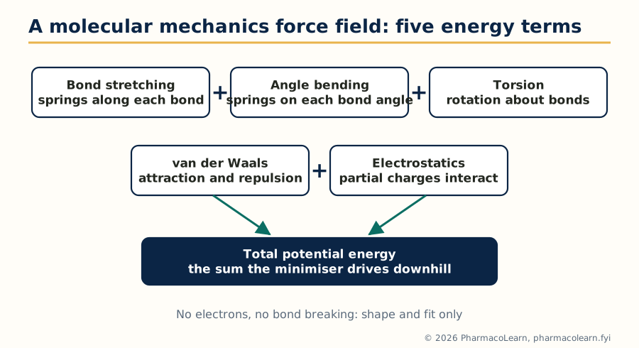
Figure: Molecular mechanics prices a structure as a sum of bond, angle, torsion, van der Waals and electrostatic terms, with no electrons anywhere in the sum.
3.2 Quantum mechanics in drug design
Quantum mechanics (QM) keeps the electrons, and with them the chemistry MM cannot see: bond breaking and making, charge transfer, polarisation, tautomer energies, reaction barriers, and the electrostatic potential surfaces from which accurate atomic charges are derived. The QM ladder is a trade of accuracy against cost. Semi empirical methods (the AM1 and PM3 family) simplify the integrals with fitted parameters and run fast enough for routine geometry and charge work on drug sized molecules. Ab initio Hartree Fock computes from first principles without fitted parameters, and density functional theory (DFT) has become the working standard for accurate geometries, energies and properties of small molecules. In drug design QM earns its cost in specific places: deriving partial charges for a force field, checking which tautomer or protonation state actually binds, modelling covalent inhibitors whose warhead reacts with the target, understanding enzyme reaction mechanisms, and computing descriptors such as HOMO and LUMO energies for electronic QSAR terms. MM and QM are also combined, QM/MM, with the reaction centre treated quantum mechanically inside a mechanically treated protein: the active site gets the physics, the rest of the protein gets the springs.
| Aspect | Molecular mechanics | Quantum mechanics |
|---|---|---|
| Treats | Atoms as balls and springs, no explicit electrons | Electrons explicitly, by approximation scheme |
| Speed | Very fast, thousands of atoms | Slow, tens to a few hundred atoms for careful work |
| Can break bonds | No | Yes |
| Needs | A force field with parameters for every atom type | A method and basis set choice |
| Typical drug design jobs | Minimisation, conformations, dynamics, docking support | Charges, tautomers, covalent warheads, reaction mechanisms |
3.3 Energy minimization methods
A built structure arrives strained: bonds stretched by the drawing, atoms overlapping. Energy minimization walks the structure downhill on the potential energy surface to the nearest comfortable geometry. The methods differ in what they know about the hill. Steepest descent follows the gradient, the direction of steepest fall, in steps: robust far from a minimum when strains are gross, but slow and zigzagging near the bottom. Conjugate gradient remembers the previous direction and combines it with the new gradient, curing most of the zigzag and becoming the usual workhorse for large systems. Newton Raphson uses the second derivative (the curvature, the Hessian matrix) as well and converges in few steps near a minimum, but the Hessian is expensive to compute and store for big systems, and the method can misbehave far from a minimum; quasi Newton variants approximate the Hessian to keep the benefit. The simplex method uses no derivatives at all, moving a geometric figure across the surface, slow but forgiving. The practical protocol is therefore staged: steepest descent first to relieve the worst strain, then conjugate gradient to finish. Every student must hold one caveat fast: minimization finds the nearest local minimum, not the lowest one on the surface; that search problem is the next section.
3.4 Conformational search: finding the shapes a molecule can take
Flexible molecules live as populations of conformations, and modeling must enumerate the plausible ones. Systematic search rotates each rotatable bond in steps (say every 30 or 60 degrees) over the full circle and keeps the combinations that survive an energy cut off: complete for small molecules, but the count explodes combinatorially, roughly the step count raised to the number of rotatable bonds, so it fails beyond a handful of rotors. Monte Carlo methods change one feature at random, accept or reject the result by an energy criterion, and sample rather than enumerate, reaching larger and more flexible molecules at the price of no guarantee of completeness. Molecular dynamics gives the molecule kinetic energy and integrates Newton's equations, so the structure wanders the surface as it would at temperature, crossing small barriers and revealing flexible regions, hinge motions and water behaviour over time; snapshots along the trajectory are the conformational sample. Simulated annealing, heating and slow cooling in silico, is the hybrid used to shake a system out of poor minima. For pharmacophore work (Unit 5) and docking, the working product is a conformational ensemble: a stored set of low energy shapes per molecule, from which the binding one is chosen.
3.5 Global minimum versus bioactive conformation
The syllabus pairs two ideas that students routinely confuse. The global minimum conformation is the single lowest energy shape of the isolated molecule. The bioactive conformation is the shape the molecule actually adopts in the binding site. They are often different, and the difference costs energy: binding spends part of its budget forcing the ligand out of its favourite shape into the bound one, a conformational strain the complex must repay with interactions. Two practical consequences follow. First, a modeling study that minimises a ligand and docks only that shape has silently assumed the two conformations coincide; flexible docking and conformational ensembles exist to avoid that assumption. Second, conformational restriction is a design strategy: if the bioactive shape is known, locking the molecule into it with a ring or a double bond pre pays the strain and often buys potency and selectivity, at the risk that the locked shape is the wrong guess. Comparing the global minimum with a proposed bioactive conformation, and counting the energy gap between them, is a standard sanity check in structure based work; gaps beyond a few kilocalories per mole make the proposed pose suspect.
3.6 Molecular docking: what it is, and how a run proceeds
Molecular docking predicts how a small molecule sits in a target's binding site, its pose, and estimates how strongly it binds, its score. It is the workhorse of structure based design and of docking based virtual screening.
1. Prepare the protein .... add hydrogens, assign protonation, repair gaps
        |
        v
2. Define the site ........ binding pocket from the bound ligand or geometry
        |
        v
3. Prepare the ligands .... 3D structures, tautomers, ionisation states
        |
        v
4. Sample poses ........... place and rotate the ligand in the pocket
        |
        v
5. Score each pose ........ estimated binding energy or fit score
        |
        v
6. Inspect and test ....... eye, interactions, then the bench decides
Preparation is where docking studies succeed or fail quietly: a histidine protonated the wrong way, a missing structural water that actually mediates binding, a ligand drawn in the wrong tautomer, each silently poisons the result. The validation every docking protocol owes is redocking: remove the ligand from an experimental complex, dock it back, and demand that the top pose reproduces the experimental one, conventionally within a root mean square deviation of about 2 Angstrom. A program that cannot redock its own answer has not earned trust on unknown ligands.
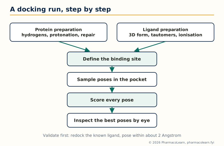
Figure: A docking run proceeds from careful preparation through sampling and scoring to inspection, and earns trust only by redocking a known ligand correctly.
3.7 Search algorithms and scoring functions
Docking divides labour between a search algorithm, which explores placements, and a scoring function, which prices them. Search strategies include systematic incremental construction, building the ligand fragment by fragment inside the pocket (the strategy of FlexX and of DOCK's anchor and grow), genetic algorithms that evolve a population of poses under selection for score (the strategy of GOLD and of AutoDock's Lamarckian variant), Monte Carlo and simulated annealing moves, and exhaustive shape matching for rigid fragments. Scoring functions come in three families. Force field based scores extend the MM energy of section 3.1 to the complex, counting van der Waals and electrostatic terms between ligand and protein. Empirical scores add up fitted contributions, a hydrogen bond term, a hydrophobic contact term, a penalty per rotatable bond, calibrated on complexes with known affinities. Knowledge based scores derive potentials from statistics of atom contacts in the structural databases. All three share known weaknesses: they rank poses within one ligand reasonably, compare different ligands shakily, treat water and protein motion crudely, and largely ignore entropy. Docking scores are therefore used to enrich a list with plausible binders and to generate binding hypotheses, not as measured affinities; the free energy methods that do better exist, at far greater cost.
3.8 Rigid, flexible and extra precision docking
| Mode | Protein | Ligand | Typical use |
|---|---|---|---|
| Rigid docking | Fixed | Fixed, one stored conformation | Very fast first pass over huge libraries |
| Flexible docking | Fixed (or partly) | Flexible, conformations generated during the run | The standard working mode for lead work |
| Extra precision (XP) docking | Fixed | Flexible, with a stricter, more physical scoring stage | Final ranking of shortlists, punishing false positives |
The syllabus's phrase extra precision docking comes from the Glide program's XP mode: after a standard precision pass, poses are rescored with a more demanding function that rewards specific motifs, such as hydrogen bonds in hydrophobic enclosures, and penalises the solvent exposed, charge mismatched poses that looser scoring lets through. The general pattern matters more than the brand: docking is run as a cascade, cheap and lenient first over millions, strict and expensive last over hundreds, a pattern Unit 5 formalises as the screening protocol.
3.9 Drug receptor interactions, in the language of docking
Docking stands or falls on the same interaction catalogue as medicinal chemistry, now with geometry attached. Hydrogen bonds are directional and short, roughly 2.5 to 3.2 Angstrom between heavy atoms, and a pose that satisfies the site's donors and acceptors usually beats one that merely fills space. Hydrophobic contacts reward burying nonpolar surface against nonpolar pocket walls, the in silico face of the log P story of Unit 1. Electrostatic interactions range from salt bridges between full charges to the weak pull of dipoles. Pi stacking and cation pi interactions organise aromatic ligands against aromatic or charged side chains. Metal coordination dominates in metalloenzyme sites, as with the zinc ion bound by inhibitors of carbonic anhydrase and of matrix metalloproteinases. And water is an honorary residue: ordered waters in a pocket may be displaced by a ligand, gaining entropy, or bridged by it, gaining enthalpy, and good protocols decide water by water which treatment applies.
3.10 Case target: DHFR and methotrexate
Dihydrofolate reductase (DHFR) reduces dihydrofolate to tetrahydrofolate, the carrier that feeds one carbon units into thymidylate and purine synthesis; block it and DNA synthesis starves. Its inhibitor family is the classical docking teaching case. Methotrexate, a folate analogue, binds DHFR extremely tightly in place of the substrate, and species selective relatives such as trimethoprim, selective for bacterial DHFR, show how small pocket differences between species are read, by eye and by docking, into selective drugs. A docking exercise on DHFR teaches the canonical lessons in one system: the pteridine ring anchors by hydrogen bonds deep in the pocket, the glutamate tail reaches toward solvent and charged residues, and the score separates substrate like poses from nonsense ones. DHFR is also a resistance lesson: point mutations in the pocket that weaken inhibitor binding while sparing substrate turnover are exactly the poses a docking program can be asked to explain.
3.11 Case targets: HMG CoA reductase, HIV protease and the cholinesterases
HMG CoA reductase catalyses the rate limiting step of cholesterol synthesis, the conversion of HMG CoA to mevalonate, and is the target of the statins. The statin pharmacophore carries an HMG like portion that occupies the HMG binding region and a rigid hydrophobic group that fits an adjacent pocket created when the enzyme closes over the inhibitor; docking into this site turns on reproducing the flap closure, a reminder that some pockets only exist in the bound state. HIV protease, a symmetric aspartic protease dimer that cleaves the viral polyprotein, was the first great triumph of structure based design: its inhibitors, beginning with saquinavir, approved in 1995 as the first protease inhibitor, were designed against the enzyme's known structure, peptidomimetic in ancestry, and anchored on interactions with the catalytic aspartates and the conserved water that bridges inhibitor to the flaps. The cholinesterases complete the syllabus set: acetylcholinesterase (AChE), which clears acetylcholine in synapses, has a deep narrow gorge with a catalytic site at its base and a peripheral site at its rim, the geography behind donepezil, whose long shape touches both sites, while butyrylcholinesterase (BChE), its plasma and brain relative, differs in gorge lining and selectivity patterns. Docking across these four target families, an oxidoreductase, a reductase of lipid metabolism, a viral protease and two hydrolases, is the syllabus telling the student that the method is general, and that each target still has to be learned on its own terms.
Unit 4: Molecular Properties and Drug Design
4.1 ADMET: why good binders fail as drugs
Ask why development candidates die and the answer, historically, was rarely potency. Compounds failed because they were not absorbed from the gut, were cleared in minutes, accumulated where they should not, or injured the liver and heart. ADMET names the five gates: Absorption, Distribution, Metabolism, Excretion and Toxicity. Predicting these properties in silico, the syllabus's first Unit 4 item, matters because of timing: a potency problem found in a screening assay costs an assay, an ADMET problem found in the clinic costs a programme. The modern discovery pipeline therefore predicts early and often, using ADMET models as filters in virtual screening and as design feedback in lead optimisation, and Unit 4 treats prediction and design together for exactly that reason.
4.2 The properties predicted, gate by gate
- Absorption: aqueous solubility, the gatekeeper property, and intestinal permeability, estimated from descriptors by models trained on cell assays such as Caco 2; log P and log D (Unit 1) feed both.
- Distribution: plasma protein binding, which sets the free fraction able to act; volume of distribution predictions; and blood brain barrier penetration models, wanted for CNS drugs and feared for others.
- Metabolism: prediction of metabolic stability, of the cytochrome P450 isoforms a compound inhibits or is cleared by, and of likely soft spots on the structure where enzymes attack; a predicted liability is a design instruction, block that position or soften it.
- Excretion: renal and biliary clearance tendencies, largely read from size, charge and lipophilicity.
- Toxicity: structural alerts for mutagenicity and reactivity, and models for specific mechanisms such as hERG potassium channel blockade, the classic cause of fatal cardiac arrhythmia surprises.
Every prediction carries an applicability domain, as in Unit 2: the model knows the chemistry it was trained on and guesses outside it.
4.3 Drug likeness rules: Lipinski and Veber
Two rule sets turn ADMET experience into numbers a chemist can apply at the drawing board. Lipinski's rule of five (1997), distilled from the property ranges of orally absorbed drugs, flags likely poor absorption or permeation when a compound has more than one of: molecular weight above 500, log P above 5, more than 5 hydrogen bond donors, more than 10 hydrogen bond acceptors. The rules are named for their multiples of five, are about oral exposure only, and carry known exceptions, notably transport substrates and most natural products; they are a warning light, not a law of nature. Veber's rules add shape and polarity: rotatable bonds of 10 or fewer and polar surface area of 140 square Angstrom or less predict good oral bioavailability across chemotypes. Both rule sets are routinely used as the first, cheapest filter in virtual screening (Unit 5), and both are exactly the kind of crude, useful model this subject teaches students to use and to doubt at the same time.
4.4 De novo design: growing a molecule inside the cavity
Ligand based methods remodel what exists; de novo design builds what does not. The programme is given the binding site, empty, and assembles a molecule inside it, atom by atom or fragment by fragment, scoring as it grows. The design cycle runs:
Analyse the cavity: size, shape, interaction hot spots
        |
        v
Place seed fragments at the hot spots
        |
        v
Grow or link fragments into complete molecules
        |
        v
Score fit, strain and synthetic accessibility
        |
        v
Chemist reviews: can it be made? is it new?
        |
        v
Synthesise a shortlist and test
Early programs such as LUDI worked by placing fragments matching the site's hydrogen bond and hydrophobic hot spots and then linking them; later systems grow chains atom by atom under genetic or Monte Carlo search. The chronic weakness of the method is the same as its charm: the computer is a more imaginative chemist than the team, and many de novo structures are unsynthesisable, unstable or absurd, so scoring includes a synthetic accessibility estimate and the chemist's veto is structural, not decorative.
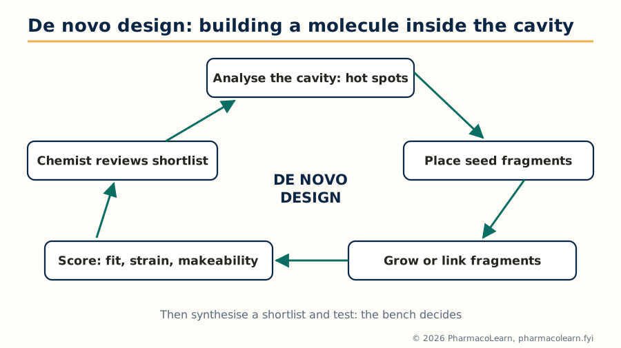
Figure: De novo design is a cycle inside the cavity, and the chemist's review step is what keeps its imagination synthesisable.
4.5 Reading a binding cavity: size and functional components
The syllabus breaks cavity analysis into three tasks, and a de novo or fragment project does them in order. Interaction analysis maps where the site makes its demands: the hydrogen bond donors and acceptors of backbone and side chains, the charged residues, the hydrophobic walls, any metal centre or ordered water; protein ligand complexes of relatives and fragment soaking experiments reveal which of these are hot spots, positions where binding energy concentrates. Cavity size prediction measures the pocket's volume and shape from the protein surface, deciding whether the site can host a drug sized molecule at all, a druggability judgement, and which direction a growing molecule can extend. Predicting the functional components of the cavity classifies each region by what a ligand should present to it: donor here, acceptor there, aromatic ring against that wall, positive charge nowhere near the acidic residue. The output is a blueprint, and sections 4.4 and 4.6 are two ways of building to it.
4.6 Fragment based drug design
Fragment based drug design (FBDD) starts from the observation that small fragments, molecular weight roughly 150 to 300, bind weakly but efficiently, and that nearly every pocket will bind some fragments at its hot spots. A fragment library of one or two thousand members is screened by sensitive methods, biophysical techniques such as NMR, surface plasmon resonance and X ray crystallography, rather than by potency assays, because fragment affinities are millimolar, not nanomolar. Crystallography then shows exactly where and how each fragment binds. Design grows the fragment, links two fragments binding side by side, or merges overlapping ones, keeping the efficient core and adding interactions, the path by which potency is built step by step. The rule of three guides library design, the fragment sized cousin of Lipinski's rules: molecular weight below 300, log P at or below 3, donors and acceptors at or below 3 each. The approach's textbook successes are real drugs: the BRAF inhibitor vemurafenib and the BCL 2 inhibitor venetoclax both began as fragment campaigns, proof that the syllabus item is a living industrial method and not a classroom curiosity.
4.7 Homology modeling: a structure for a protein that has none
Docking and de novo design need a three dimensional target, and for many targets no experimental structure exists. Homology modeling builds one from a relative: if the target's amino acid sequence resembles that of a protein whose structure is known, the template, the target almost certainly folds the same way, because structure is more conserved than sequence. The workflow:
Target sequence
      |
      v
Template search (sequence alignment against known structures)
      |
      v
Align target to template, carefully, around conserved regions
      |
      v
Build the backbone on the template, model the variable loops
      |
      v
Place side chains, minimise, refine
      |
      v
Validate the model, then use it for docking or design
Reliability tracks sequence identity: above about 50 percent identity, models are generally trustworthy in the core; between 30 and 50 percent, usable with care; below about 30 percent, the twilight zone, where alignment errors dominate and models mislead as often as they guide. The conserved core inherits the template's backbone; insertions and deletions fall in surface loops, which are therefore the least reliable parts, and, inconveniently, often line binding sites.
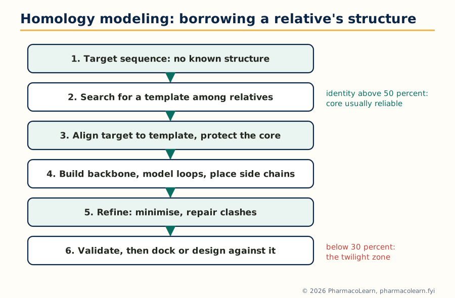
Figure: Homology modeling borrows a relative's fold; reliability is set at the template step and proved at the validation step.
4.8 Validating the model before trusting it
A homology model is a hypothesis and is examined like one. The Ramachandran plot checks that backbone torsion angles fall in the sterically allowed regions where real proteins live; outliers mark strained, probably wrong, segments. Knowledge based energy and statistical profiles compare the model's residue environments with those of experimental structures, flagging buried charges and exposed hydrophobics that nature avoids. Active site sanity is the pragmatic test: residues known from mutagenesis or from family conservation to matter must land where the model needs them, and known ligands should dock into the model the way they dock into relatives. The deliverable of Unit 4, taken whole, is a judgement call this course trains deliberately: which computational evidence, ADMET prediction, de novo sketch, fragment hit or homology model, is strong enough to spend synthesis on.
Unit 5: Pharmacophore Mapping and Virtual Screening
5.1 The pharmacophore concept
Strip a family of active molecules down to the arrangement that activity cannot live without and you have a pharmacophore: the spatial arrangement of features, hydrogen bond donors and acceptors, charged groups, aromatic rings, hydrophobic regions, that a molecule must present, in the right geometry, to bind its target. The word descends from Ehrlich's side chain ideas and was sharpened by generations of medicinal chemists comparing active analogues; the modern statement, in the IUPAC sense, is that a pharmacophore is the ensemble of steric and electronic features necessary for optimal interaction with a specific target and for triggering or blocking its response. Two properties of the concept matter for everything after. A pharmacophore is an abstraction: it names features and distances, not atoms, so chemically different scaffolds can match the same pharmacophore, which is why the method finds new chemotypes. And it is a hypothesis: built from the molecules that taught it, falsifiable by the next assay.
5.2 Pharmacophore features and their identification
The working feature set is short and standard:
- Hydrogen bond donor: a hydroxyl, amine or amide NH, drawn at the donor heavy atom, often with a projected point where the partner should sit.
- Hydrogen bond acceptor: a carbonyl oxygen, ether oxygen or ring nitrogen, again with a direction, because hydrogen bonds have geometry.
- Positive and negative ionisable features: a basic nitrogen protonated at physiological pH, a carboxylate, placed where a salt bridge is wanted.
- Hydrophobic feature: an aromatic ring or an alkyl cluster that must sit in a nonpolar pocket.
- Aromatic ring feature: where flat, pi stacking contact is the requirement, distinct from mere bulk.
- Excluded volumes: regions where atoms are forbidden because the protein is there, added when a model keeps proposing clashes.
Identification proceeds by aligning the active molecules and asking what they share: the features that recur, at consistent mutual distances and angles, across actives while absent or misplaced in inactives, form the model. Tolerances are part of the model; a feature sphere of generous radius admits near matches, a tight one admits only close family.
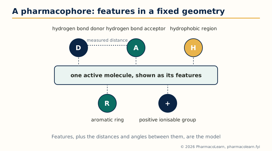
Figure: Five common feature types held at measured distances: the abstraction that lets new scaffolds match an old binding idea.
5.3 Building the model: ligand based and structure based
A ligand based pharmacophore is derived from a set of active molecules alone, as in section 5.2: the method of choice when the target structure is unknown, and dependent on the alignment of the actives, which in turn depends on their conformations, the subject of section 5.4. A structure based pharmacophore is derived from a protein ligand complex or an empty binding site: the pocket's donors, acceptors and hydrophobic patches (the cavity analysis of section 4.5) are converted directly into features, with excluded volumes read off the protein surface. The two routes are complementary and often combined: a structure based model disciplined by which of its features the known actives actually use. Either way, the model is then scored against databases of known actives and inactives; a model that retrieves the actives while rejecting the inactives has earned screening work.
5.4 Conformational search in pharmacophore mapping
A pharmacophore is a statement about three dimensional geometry, so mapping one from flexible molecules raises the question of section 3.4 in a sharper form: which conformation of each active molecule is the binding one? Conformational search used in pharmacophore mapping therefore generates, for every training molecule, an ensemble of low energy conformations by systematic rotation, Monte Carlo sampling or dynamics, and the mapping process tries the ensemble, not a single shape, looking for a feature arrangement that some conformation of every active can present. The discipline is energetic: conformations far above the global minimum (section 3.5) are implausible binding candidates and are cut, which both speeds the search and keeps the model honest. A pharmacophore built from strained, impossible conformations will screen for molecules that cannot adopt it, an elegant route to an empty hit list.
5.5 Virtual screening: the idea and the cascade
Virtual screening is the in silico counterpart of high throughput screening: instead of robotically assaying a physical library, a computational protocol scores a database of structures and ranks them, so that the fraction physically tested is the fraction most likely to be active. Databases run to millions of commercially available or enumerated compounds; the output is not drugs but hits, weak, real binders to be confirmed and optimised. Because no single method is both fast enough for millions and accurate enough to trust, practical screening is a cascade: cheap filters first, expensive physics last, each stage shrinking the list by orders of magnitude. The enrichment that justifies the whole exercise is measured against random selection: a good protocol concentrates the true actives into the top fraction of its ranking far beyond chance.
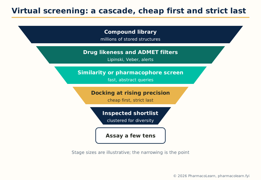
Figure: The screening cascade spends cheap computation on millions so that expensive computation, and finally bench assays, are spent on tens.
5.6 Similarity based methods: fingerprints and the Tanimoto coefficient
The oldest screening idea is the similarity principle: molecules that look alike tend to act alike. Similarity searching takes a known active as the query and ranks a database by resemblance. Resemblance is computed on fingerprints, bit strings in which each bit records the presence of a structural feature, a bond path, an atom environment or a substructure. The standard comparator is the Tanimoto coefficient: the number of bits set in both fingerprints divided by the number set in either, ranging from 0, nothing shared, to 1, identical fingerprints. A worked example: molecule A sets 12 bits, molecule B sets 10, and 7 bits are set in both; the Tanimoto coefficient is 7 divided by (12 plus 10 minus 7), that is 7 divided by 15, about 0.47. Working thresholds depend on the fingerprint, but similarities around 0.85 and above on common fingerprints usually mean close analogues, while the interesting scaffold hops hide lower, among the 0.6 to 0.8 neighbours that share the pharmacophore but not the skeleton. The method's weakness is written into its principle: it finds more of what you already know, and it is blind when activity turns on a feature the fingerprint does not encode.
5.7 Pharmacophore based screening
Pharmacophore based screening searches a database of precomputed conformations for molecules that can present the model's features within their tolerances and outside its excluded volumes. Because the query is abstract, the hits are structurally diverse by construction: a benzene query never appears, only the geometry of features, so a new scaffold that happens to hold a donor, an acceptor and a ring at the model's distances surfaces alongside the usual analogues. This is the standard route to scaffold hopping, changing the core of a series while keeping its binding logic, valuable when the old core is patented, toxic or intractable. The screen's quality is the model's quality: models built on a single chemotype, with features set too loosely, retrieve thousands of false positives, and models set too tightly retrieve only the training family, so model validation on actives and decoys, as in section 5.3, precedes any serious screen.
5.8 Structure based virtual screening protocols
A structure based in silico virtual screening protocol, the syllabus's closing topic, runs docking (Unit 3) as the screen. A defensible protocol reads as a checklist:
Database of compounds, prepared: 3D, tautomers, charges, duplicates out
        |
        v
Drug likeness and property filters (Lipinski, Veber, ADMET alerts)
        |
        v
Fast docking of the whole library, lenient scoring
        |
        v
Top fraction re-docked at higher precision (extra precision mode)
        |
        v
Consensus scoring and interaction checks (key hydrogen bonds made?)
        |
        v
Visual inspection of the shortlist, clustering for diversity
        |
        v
Order or synthesise a few tens of compounds, assay, confirm hits
Each step is a decision a student should be able to defend: the protein preparation and redocking validation of section 3.6; the choice of filters and the actives they might wrongly kill; the enrichment expected at each cut; and the final, essential step off the computer, the assay, without which a virtual hit is only a well formatted opinion. Known traps complete the syllabus: docking into the wrong protonation state, trusting scores as energies, screening databases whose stored stereochemistry is undefined, and forgetting that frequent hitters, reactive and aggregating compounds, game assays as happily as they game scoring functions.
5.9 What this subject adds up to
The five units form one workflow. Parameters turn structures into numbers (Unit 1); QSAR turns numbers into equations and teaches suspicion of them (Unit 2); modeling and docking give the numbers a three dimensional stage (Unit 3); property prediction and the design methods decide what is worth building, including building the target itself when nature has not published it (Unit 4); and pharmacophores with virtual screening scale the whole logic to millions of molecules (Unit 5). The computer's verdict is always a shortlist and a hypothesis. The laboratory still casts the deciding vote, but it votes on a much better ballot.
Frequently Asked Questions
Q: What is computer aided drug design (CADD) in one line? A: CADD is the use of computational techniques, QSAR, modeling, docking, property prediction and virtual screening, to decide which molecules are worth making and testing in drug discovery.
Q: What is the difference between SAR and QSAR? A: SAR is a qualitative account of how structural changes affect activity, while QSAR expresses activity as a mathematical equation in physicochemical parameters, so it can predict untested compounds and be statistically tested.
Q: Why does QSAR use log (1/C) instead of the raw activity? A: Because binding free energy is proportional to the logarithm of potency, so substituent effects add up linearly on the log scale, which is what regression equations assume.
Q: What does a negative coefficient on (log P) squared in a Hansch equation mean? A: It means activity is parabolic in lipophilicity: it rises to an optimum log P0 and then falls, because very lipophilic compounds dissolve poorly and get trapped in membranes instead of reaching the target.
Q: How do Hansch and Free Wilson analysis differ? A: Hansch analysis regresses activity on physicochemical parameters such as log P and sigma and can predict new substituents, while Free Wilson analysis assigns a fixed activity contribution to each substituent seen in the series and can only rank substituents already tested.
Q: Why is q squared more important than r squared for judging a QSAR model? A: r squared measures fit to the compounds used in building the model and can be inflated by adding terms, whereas q squared comes from cross validation on held out compounds and measures whether the model actually predicts.
Q: What is the difference between the global minimum and the bioactive conformation? A: The global minimum is the lowest energy shape of the free molecule, while the bioactive conformation is the shape it adopts in the binding site; the energy gap between them is a strain the binding interactions must repay.
Q: What do a docking search algorithm and a scoring function each do? A: The search algorithm explores the ligand's positions, orientations and conformations in the binding site, and the scoring function estimates the quality or binding strength of each pose so the poses can be ranked.
Q: What is the point of redocking when validating a docking protocol? A: Redocking removes a ligand from its experimental complex and docks it back; if the program cannot reproduce the known pose, usually within about 2 Angstrom RMSD, its poses for unknown ligands should not be trusted.
Q: When is homology modeling reliable enough to use for drug design? A: As a working rule, models built from templates with more than about 50 percent sequence identity are generally reliable in the core, models at 30 to 50 percent need care and validation, and below about 30 percent the alignment errors usually dominate.
Complete MPC203T notes, all 5 units in one PDF, free to keep.
Other M.Pharm subjects: MPH101T · MPC101T · MPL101T · MPH102T · MPH103T · MPH104T · MPL102T · MPL103T · MPL104T · MPC102T · MPC103T · MPC104T · MPH201T · MPH202T · MPH203T · MPH204T · MPC201T · MPC202T · MPC203T · MPC204T · M.Pharm