
MPC201T — Advanced Spectral Analysis
4 hrs/week, 4 credits, 60 hours, 100 marks (75 end semester + 25 sessional). Notes follow the M.Pharm syllabus, unit by unit.
MPC201T Advanced Spectral Analysis notes for M.Pharm Semester 2 Pharmaceutical Chemistry: Woodward-Fieser rules, ATR-IR and IR interpretation, 2-D NMR with COSY, NOESY, HETCOR and INADEQUATE, mass fragmentation rules and hyphenated techniques, with free unit wise PDF downloads on PharmacoLearn.
Units in this subject
- Unit 1 — UV and IR spectroscopy: Woodward-Fieser rules for 1,3-butadienes, cyclic dienes and alpha,beta-unsaturated carbonyl compounds, interpretation of enones, ATR-IR, IR interpretation of organic compounds
- Unit 2 — NMR spectroscopy: 1-D and 2-D NMR, NOESY and COSY, HETCOR, INADEQUATE techniques, interpretation of organic compounds
- Unit 3 — Mass spectroscopy: mass fragmentation and its rules, fragmentation of alcohols, amines, carbonyl groups and alkanes, metastable ions, McLafferty rearrangement, ring rule, isotopic peaks, interpretation of organic compounds
- Unit 4 — Chromatography: principle, instrumentation and applications of GC-MS, GC-AAS, LC-MS, LC-FTIR, LC-NMR, CE-MS, HPTLC, supercritical fluid chromatography, ion chromatography, ion exclusion chromatography and flash chromatography
- Unit 5 — Thermal methods of analysis (DSC, DTA, TGA), Raman spectroscopy, and radioimmunoassay: biological standardization, bioassay, ELISA, radioimmunoassay of digitalis and insulin
Download MPC201T PDF Notes
Free PDFs for this subject, one per unit:
Advanced Spectral Analysis, subject code MPC201T, is a core Semester 2 subject of M.Pharm Pharmaceutical Chemistry. It carries 4 credits and 60 hours of theory, taught at 4 hours per week, for 100 marks.
Semester 1's Modern Pharmaceutical Analytical Techniques (MPC101T) taught how each instrument works. This subject teaches the skill the instruments exist for: interpretation. Unit 1 turns UV and IR spectroscopy into a predictive and reading discipline, the Woodward-Fieser rules for calculating the absorption maximum of dienes and enones, ATR-IR, and a systematic routine for reading an infrared spectrum. Unit 2 moves NMR into two dimensions: COSY, NOESY, HETCOR and INADEQUATE, the experiments that trace which proton couples to which, which proton sits on which carbon, and how the carbon skeleton itself is connected. Unit 3 treats the mass spectrum as a fragmentation puzzle governed by rules: alpha cleavage, the McLafferty rearrangement, metastable ions, the ring rule and isotopic patterns. Unit 4 couples separation to identification in the hyphenated techniques, GC-MS, LC-MS, LC-NMR, CE-MS and their companions, with HPTLC, supercritical fluid, ion and flash chromatography. Unit 5 covers the supporting physical and biological methods: DSC, DTA and TGA, Raman spectroscopy, and the immunoassay family, ELISA and the radioimmunoassays of insulin and digitalis. A student who completes this subject should be able to take an unknown compound's UV, IR, NMR and mass spectra and argue, spectrum by spectrum, to a structure that fits all four.
Unit 1: UV and Infrared Spectroscopy: Woodward-Fieser Rules, ATR-IR and IR Interpretation
1.1 Where this subject begins: from instruments to interpretation
Every technique in this unit measures the same event from a different side: a molecule absorbing energy of a particular wavelength and changing state. UV and visible light drive electronic transitions, infrared light drives vibrations, radiofrequency radiation flips nuclear spins in NMR, and mass spectrometry, the exception, uses no radiation at all and instead weighs ions. Interpretation is the reverse journey: from the positions and shapes of absorptions back to the structural features that caused them.
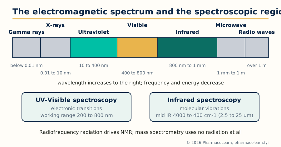 Figure: The spectroscopic regions. UV and IR interpretation dominate this unit; NMR and MS complete the evidence in Units 2 and 3.
The working discipline of the whole subject can be stated now. No single spectrum proves a structure. UV speaks about conjugation, IR about functional groups, NMR about the proton and carbon framework, and MS about molecular weight and fragmentable subunits. A structure is accepted when it is the only reasonable one consistent with all the evidence, and the exam problems in this subject are built exactly that way.
1.2 UV-Visible spectroscopy at the advanced level
The electronic transitions were introduced in MPC101T; what matters for interpretation is their ranking. In decreasing order of energy the transitions run sigma to sigma star (far UV, below the working range), n to sigma star (saturated compounds with heteroatoms, weak), pi to pi star (alkenes, dienes, aromatics and carbonyls, strong, molar absorptivity typically in the thousands to tens of thousands) and n to pi star (carbonyls and other unsaturated heteroatom groups, weak and symmetry forbidden, absorptivity of the order of 10 to 100). Two consequences follow.
First, the intense pi to pi star band of a conjugated system is the analyst's handle: its position moves predictably with the length and substitution of the conjugated system, which is exactly what the Woodward-Fieser rules of the next sections quantify. Second, solvent polarity moves the two band types in opposite directions. A polar solvent stabilises the n orbital of a carbonyl, so n to pi star bands shift to shorter wavelength (a blue or hypsochromic shift) in polar solvents, while pi to pi star bands, whose excited state is more polar than the ground state, shift to longer wavelength (a red or bathochromic shift). Watching a band move when the solvent is changed is therefore a quick experimental test of which transition it is.
The vocabulary of shifts is used constantly in interpretation and should be exact: bathochromic (to longer wavelength), hypsochromic (to shorter), hyperchromic (more intense) and hypochromic (less intense). A fifth practical point: UV evidence is corroborative, never decisive on its own. A band near 254 nm with high intensity says "conjugated or aromatic system present"; it cannot say which one. That is why this subject always pairs UV with IR, NMR and MS.
1.3 The Woodward-Fieser rules for dienes
Woodward, and later Fieser, noticed that the pi to pi star maximum of a conjugated diene can be predicted by addition. Start from a base value that depends on the diene's geometry, add a fixed increment for every structural feature present, then correct for the solvent. Two base values cover dienes:
- 214 nm for an acyclic diene, or a heteroannular diene, one whose two double bonds lie in different rings.
- 253 nm for a homoannular diene, one whose two double bonds lie in the same ring (a 1,3-cyclohexadiene type system). The higher base value reflects the fixed cisoid geometry, which conjugates more effectively.
The increments (each counted once per feature) are: alkyl substituent or ring residue on the diene system, +5 nm; an exocyclic double bond (a double bond of the diene sticking out of a ring, one carbon in the ring and one outside), +5 nm; a further double bond extending the conjugation, +30 nm; and auxochromes attached directly to the diene carbons: alkoxy (-OR) +6 nm, thioether (-SR) +30 nm, chloro or bromo +5 nm, and dialkylamino (-NR2) +60 nm. Solvent corrections are made relative to ethanol: water +8 nm, methanol 0, chloroform -1 nm, dioxane -5 nm, ether -7 nm and cyclohexane or hexane -11 nm. Predictions within about 5 nm of the observed value count as agreement.
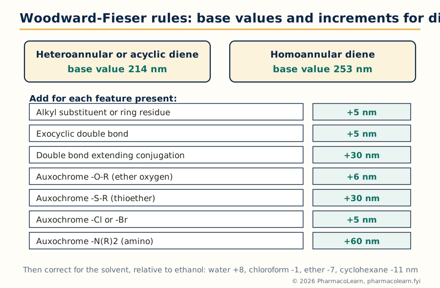 Figure: The diene rules at a glance. Base value, plus increments, plus solvent correction, gives the predicted absorption maximum.
1.4 Worked diene calculations
Example 1, an acyclic diene: 2,4-hexadiene. Base value for an acyclic diene 214 nm; two alkyl substituents (the two terminal methyl groups), 2 x 5 = 10 nm; total calculated 224 nm. Observed 227 nm. Agreement is good, and the calculation confirms the conjugated diene rather than two isolated double bonds, whose pi to pi star bands would lie below the working range.
Example 2, a homoannular steroidal diene: ergosterol. The conjugated diene of ergosterol (double bonds at 5-6 and 7-8) lies within ring B, so it is homoannular: base 253 nm. Ring residues on the diene carbons: C-5 carries two ring residues and C-8 carries two, total 4 x 5 = 20 nm. Both double bonds are exocyclic to a neighbouring ring (the 5-6 bond to ring A, the 7-8 bond to ring C), 2 x 5 = 10 nm. Total calculated 253 + 20 + 10 = 283 nm. Observed 282 nm. This is the classic demonstration that the rules work on real drug like molecules: a student given only the structure predicts the spectrum of a sterol within 1 nm.
Two habits make these calculations reliable in examinations. First, count ring residues carefully: a ring residue is any carbon substituent on a diene carbon that is part of a ring, and ring junction carbons often carry two. Second, an exocyclic double bond is counted once for each ring to which it is exocyclic. Steroidal dienes fail more students on counting than on chemistry.
1.5 The Woodward-Fieser rules for alpha,beta-unsaturated carbonyl compounds
Enones have their own base values and increments, and the same additive logic. The base value depends on the carbonyl class and ring size:
| Parent chromophore | Base value (nm) |
|---|---|
| Acyclic alpha,beta-unsaturated ketone | 215 |
| Six membered cyclic enone | 215 |
| Five membered cyclic enone | 202 |
| Alpha,beta-unsaturated aldehyde | 210 |
| Alpha,beta-unsaturated carboxylic acid or ester | 195 |
The increments are position dependent, which is what makes enone calculations a genuine test of structure reading:
| Feature | Increment (nm) |
|---|---|
| Alkyl group or ring residue at the alpha carbon | +10 |
| Alkyl group or ring residue at the beta carbon | +12 |
| Alkyl group or ring residue at the gamma or delta carbon | +18 |
| Exocyclic double bond | +5 |
| Double bond extending conjugation | +30 |
| Homoannular diene component within the enone | +39 |
| Hydroxyl at alpha / beta | +35 / +30 |
| Alkoxy at alpha / beta / delta | +35 / +30 / +31 |
| Chloro at alpha / beta | +15 / +12 |
| Bromo at alpha / beta | +25 / +30 |
| Dialkylamino at beta | +95 |
Solvent corrections for enones, again relative to ethanol or methanol (0): water +8, chloroform -1, dioxane -5, ether -7, hexane or cyclohexane -11 nm. The alpha and beta positions are counted from the carbonyl carbon: the carbon adjacent to C=O is alpha, the next is beta, and an extended system continues gamma, delta.
1.6 Worked enone calculations, and reading enones from spectra
Example 1: mesityl oxide (4-methylpent-3-en-2-one). An acyclic enone: base 215 nm. The beta carbon carries two methyl groups, 2 x 12 = 24 nm. Calculated 239 nm; observed 235 nm. The beta disubstitution is read directly off the size of the shift from base value.
Example 2: cholest-4-en-3-one. The enone sits in a six membered ring (ring A of the steroid): base 215 nm. The beta carbon (C-5, the ring junction) carries two ring residues, 2 x 12 = 24 nm. Calculated 239 nm; observed 241 nm. Note how the same arithmetic distinguishes this common steroidal enone pattern from a five membered ring enone, whose base value is 13 nm lower: ring size is encoded in the spectrum.
Interpretation runs the calculation backwards. An unknown showing an intense band near 240 nm whose Woodward-Fieser estimate for a proposed enone structure agrees within a few nm supports the enone; if the estimate for the proposed structure is 215 nm but the band sits at 250 nm, the structure is wrong somewhere, usually in the substitution pattern at the beta carbon. Two cautions complete the topic. Strong steric twisting of the conjugated system out of planarity (heavily hindered enones) lowers intensity and can shift the band, because conjugation needs coplanarity. And the weak n to pi star band of the carbonyl, near 300 to 350 nm with absorptivity under 100, should still be visible for an enone and moves to shorter wavelength in polar solvents, a useful confirmation that the chromophore really contains C=O.
1.7 Reading an infrared spectrum: the correlation chart
An infrared spectrum is read in two zones. The functional group region, roughly 4000 to 1500 cm-1, holds the stretching vibrations whose frequencies are characteristic of particular bonds and groups: this is where O-H, N-H, C-H, triple bonds, C=O and C=C announce themselves. The fingerprint region, roughly 1500 to 600 cm-1, holds coupled skeletal vibrations and bending modes that are unique to the whole molecule: useless for naming groups, decisive for confirming identity against a reference spectrum.
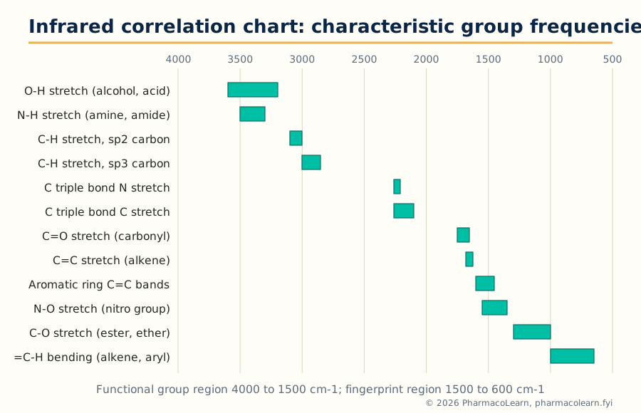 Figure: The correlation chart. Every band in the functional group region should be assigned to a row of this chart before any structure is proposed.
The chart is used with three refinements that separate interpretation from mere band spotting.
- Position is evidence about environment, not just identity. A carbonyl at 1715 cm-1 is an ordinary saturated ketone; conjugation with a double bond or ring lowers it to about 1685 cm-1; a strained four membered ring ketone rises towards 1780 cm-1; an amide, whose carbonyl is weakened by nitrogen lone pair donation, falls to about 1650 cm-1. Hydrogen bonding lowers and broadens O-H (sharp free O-H near 3600 cm-1, broad associated O-H 3200 to 3400 cm-1, the very broad envelope of a carboxylic acid dimer spanning 3300 to 2500 cm-1).
- Intensity and shape carry information. Carbonyl bands are strong; alkene C=C bands are weak to medium and vanish for symmetrically substituted double bonds; the aldehyde C-H pair near 2820 and 2720 cm-1 is weak but diagnostic; aromatic rings declare themselves by the pair of bands near 1600 and 1500 cm-1 plus the substitution pattern bands between 900 and 650 cm-1.
- Absence is evidence too. No band in the 1850 to 1650 cm-1 region means no carbonyl of any kind, which can eliminate half the candidate structures at a stroke. No broad band above 3100 cm-1 argues against O-H and N-H. A disciplined interpreter lists the absences beside the presences.
1.8 ATR-IR: infrared without sample preparation
In attenuated total reflectance, the infrared beam does not pass through the sample at all. It travels inside a crystal of high refractive index (diamond, zinc selenide or germanium) and is totally internally reflected at the crystal surface. At each reflection an evanescent wave extends a short distance, of the order of 0.5 to 2 micrometres depending on wavelength, crystal and angle, into the sample pressed against the surface. Where the sample absorbs, the reflected beam is attenuated at that wavenumber, and the detector records an absorption like spectrum after as many reflections as the crystal geometry provides.
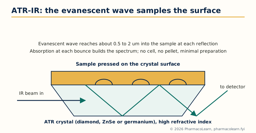 Figure: ATR geometry. The beam never crosses the bulk sample; the spectrum comes from a surface layer about a micrometre deep.
Three practical consequences explain why ATR has displaced the KBr pellet for routine work. There is almost no sample preparation: a solid, powder, paste, film or liquid is simply pressed into contact. Water, the enemy of transmission IR, is tolerable because the effective path length is micrometres, so aqueous and biological samples become measurable. And the spectrum is a surface spectrum, which is a limitation to remember with coated tablets or oxidised surfaces: ATR reports the outermost micrometre, not the bulk. Two honest caveats complete the picture: band intensities in ATR grow relatively stronger at low wavenumber than in transmission spectra (penetration depth rises with wavelength), so library matching works best against ATR libraries, and poor crystal contact gives weak spectra, which is why ATR accessories carry a pressure clamp.
1.9 A systematic routine for IR interpretation
Guessing from one familiar band is the commonest cause of wrong identifications. The routine below, applied in order, converts IR interpretation into a procedure.
START: note the physical state and how the spectrum was recorded
  |
  v
1. Carbonyl present? Look at 1850 to 1650 cm-1
   - strong band: assign the class by position
     (anhydride pair, ester 1735, aldehyde 1725, ketone 1715,
      acid 1710, amide 1650 cm-1, adjusted for conjugation/strain)
   - no band: no C=O; rule out acids, esters, ketones, amides
  |
  v
2. Above 3000 cm-1: broad 3200 to 3400 = associated O-H;
   very broad 2500 to 3300 = acid O-H; sharp 3600 = free O-H;
   3300 to 3500 pattern = N-H (one band 2 deg, two bands 1 deg amine)
  |
  v
3. C-H pattern: above 3000 = unsaturated or aromatic C-H;
   below 3000 = aliphatic; 2820 and 2720 pair = aldehyde C-H
  |
  v
4. Triple bonds and cumulenes: 2100 to 2260 cm-1 (nitrile, alkyne)
  |
  v
5. C=C and ring bands: 1620 to 1680 alkene; 1600 and 1500 aromatic;
   nitro pair near 1550 and 1370; C-O region 1000 to 1300
  |
  v
6. Fingerprint: substitution pattern 650 to 900 cm-1; compare
   the whole region against reference spectra for final identity
  |
  v
STATE: groups present, groups absent, and what remains undecided
Worked example. An unknown liquid shows: strong band at 1700 cm-1; two weak bands at 2820 and 2720 cm-1; medium bands at 1600 and 1500 cm-1; bands at 760 and 700 cm-1; nothing broad above 3100 cm-1. Reading in order: a carbonyl is present at the conjugated position (1700, lowered from 1715 by conjugation); the 2820/2720 pair identifies an aldehyde; 1600 and 1500 say aromatic ring; 760 and 700 cm-1 are the classic pair for a monosubstituted benzene; no O-H. Conclusion: benzaldehyde, C6H5CHO, consistent with every observation. Note that the answer was assembled from five independent observations, no one of which would have sufficed alone.
1.10 What UV and IR together settle
Close the unit by fixing the division of labour. UV answers one question well: how far does the conjugated system extend, and how is it substituted (quantitatively, through Woodward-Fieser). IR answers a different one: which functional groups are present, and in what environment. Neither sees the carbon skeleton's connectivity or the molecular weight; those are the business of NMR and MS. When an exam problem gives all four spectra, the intended order of attack is usually molecular formula and unsaturation count from MS, functional groups from IR, chromophore check from UV, and the framework from NMR. Units 2 and 3 now supply the second half of that method.
Unit 2: NMR Spectroscopy: 1-D and 2-D Techniques and Interpretation
2.1 The 1-D experiments this unit builds on
One dimensional NMR was covered in MPC101T: the proton spectrum (chemical shift, integration, multiplicity from spin-spin coupling) and the proton decoupled carbon spectrum, in which each chemically distinct carbon gives one line. Two 1-D companions are assumed knowledge for everything that follows. DEPT editing sorts carbon signals by the number of attached protons: in DEPT-90 only CH appears; in DEPT-135 CH and CH3 point up and CH2 points down; quaternary carbons are absent from all DEPT spectra and are found by subtraction from the broadband spectrum. Routine working values for carbon shifts: carbonyl carbons 160 to 220 ppm, aromatic and alkene carbons 100 to 160 ppm, carbons bearing oxygen or nitrogen 50 to 100 ppm, and ordinary alkyl carbons 10 to 50 ppm.
What 1-D spectra cannot do is tell the analyst which signal belongs next to which. A proton spectrum of a moderately complex drug molecule is a crowd of overlapping multiplets: shifts say what kind of environment each proton sits in, couplings hint at neighbours, but the map of connections is missing. Two dimensional NMR exists to draw that map.
2.2 Chemical shift maps for proton and carbon
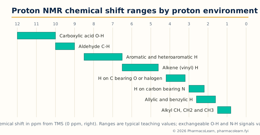 Figure: Proton shift ranges. A signal's position is the first hypothesis about its environment; 2-D experiments then test the hypothesis.
The chart is used actively, not decoratively. A three proton singlet at 3.9 ppm is a methoxy group on an aromatic ring until proved otherwise; a one proton signal near 9.8 ppm that vanishes on deuterium oxide shake was an aldehyde or an exchangeable proton, and the shake distinguishes them (an aldehyde C-H does not exchange). Exchangeable protons (O-H, N-H, S-H) give broad, concentration dependent signals that disappear on D2O exchange, while carbon bound protons keep fixed shifts: this single experiment resolves whole classes of assignment doubt, and it costs one drop of heavy water.
2.3 Why a second dimension: the 2-D experiment
A 2-D NMR spectrum spreads the information onto a plane. One axis (F2) is the ordinary chemical shift scale of the detected nucleus; the second axis (F1) is the shift scale of a second nucleus, or of the same nucleus in an earlier part of the experiment. Peaks on the diagonal of a homonuclear experiment correspond to the 1-D spectrum itself. The cross peaks off the diagonal are the new information: a cross peak at coordinates (shift A on F1, shift B on F2) states that nucleus A and nucleus B are connected in a defined way, by coupling through bonds in COSY, by closeness in space in NOESY, or by a direct carbon-proton bond in HETCOR. Choosing an experiment is choosing which kind of connection to interrogate.
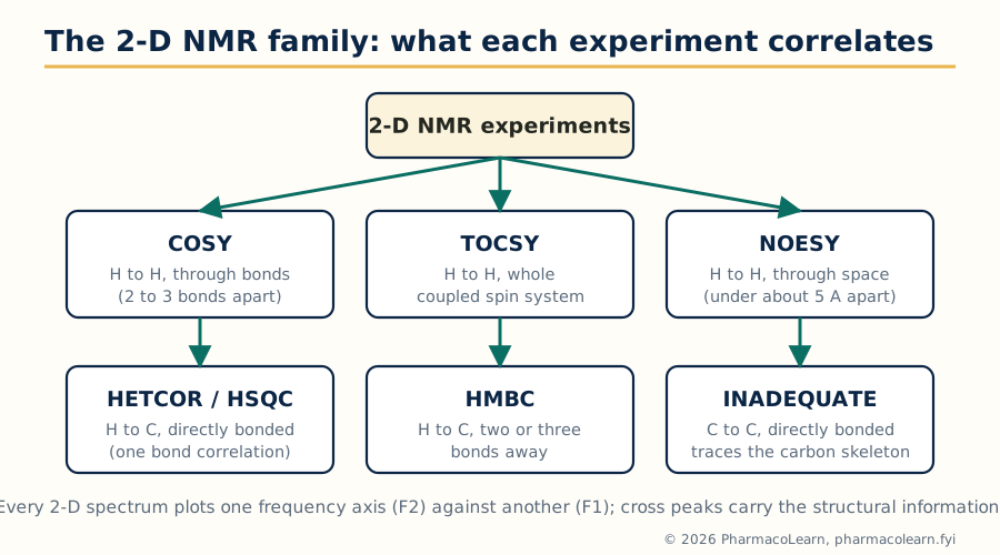 Figure: The 2-D family. Every experiment answers exactly one kind of connectivity question; interpretation is largely a matter of asking them in the right order.
2.4 Coupling constants as structural evidence
Before the 2-D experiments, one 1-D quantity deserves its own section because the 2-D spectra lean on it: the coupling constant J, measured in hertz and independent of the spectrometer's field strength. Standard working values:
| Coupling situation | Typical J (Hz) | Structural message |
|---|---|---|
| Geminal, two protons on one sp3 carbon (2J) | 12 to 15 | A CH2 group with diastereotopic protons |
| Vicinal, protons on adjacent carbons (3J) | 6 to 8 | Neighbouring CH groups; value follows dihedral angle |
| Alkene cis (3J) | 6 to 12, about 10 | Cis configured double bond |
| Alkene trans (3J) | 12 to 18, about 17 | Trans configured double bond |
| Aromatic ortho (3J) | 7 to 10 | Adjacent ring protons |
| Aromatic meta (4J) | 2 to 3 | Ring protons with one carbon between |
| Aromatic para (5J) | 0 to 1 | Opposite ring protons, often unresolved |
| Allylic (4J) | 1 to 3 | Proton allylic to a double bond |
The vicinal value carries stereochemistry through the Karplus relationship: a dihedral angle near 180 degrees (antiperiplanar, as in axial-axial protons of a cyclohexane chair) gives a large 3J of 10 to 13 Hz, while a gauche angle near 60 degrees gives 2 to 5 Hz. Sugars and steroidal systems are routinely assigned from these numbers alone. The cis and trans alkene values settle double bond geometry in one glance, a question no other routine spectrum answers as cheaply.
2.5 COSY: tracing coupled protons
In a COSY (correlation spectroscopy) experiment, both axes are the proton shift scale. A cross peak joins two proton signals that share a coupling: they are geminal partners or, far more usefully, vicinal neighbours on adjacent carbons. The spectrum is symmetric about the diagonal, so every connection appears twice.
Reading COSY is a walking exercise. Start at an unmistakable signal, an aldehyde proton, an isolated methyl singlet's neighbour, a distinctive downfield proton. Find its cross peaks: each one names a coupled partner. From that partner, find the next cross peaks, and so on, walking along the chain of coupled protons until the walk stops at a heteroatom, a quaternary carbon or a terminal methyl. Each uninterrupted walk traces one spin system, one connected run of CH and CH2 groups.
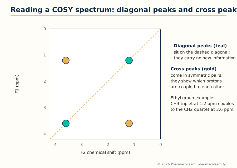 Figure: COSY logic in miniature. The ethyl group's two signals share exactly one pair of cross peaks; that pair is the entire proof that CH3 and CH2 are neighbours.
The common errors are worth naming. Long range couplings (allylic, aromatic meta) also give weak cross peaks, so a cross peak proves coupling, not always direct neighbourhood; intensity and the 1-D multiplicities arbitrate. And COSY cannot cross a break in the coupling network: an ether oxygen, an ester linkage or a quaternary carbon stops every walk, which is precisely why the heteronuclear experiments of section 2.7 exist.
2.6 TOCSY and NOESY: whole spin systems, and through space contacts
TOCSY (total correlation spectroscopy) extends COSY's idea. During its mixing period, magnetisation is relayed from proton to coupled proton along the whole network, so every proton of a spin system shows cross peaks to every other proton of the same system, not only to its immediate neighbours. In a sugar ring or an amino acid side chain, one TOCSY row displays the entire residue's protons at once, which is why TOCSY is the workhorse of peptide and carbohydrate assignment.
NOESY (nuclear Overhauser effect spectroscopy) is the odd one out: its cross peaks arise not from bonds but from the nuclear Overhauser effect, dipolar relaxation between protons close in space, effective only under about 5 angstroms. A NOESY cross peak therefore reports proximity, and its classic uses are stereochemical: cis substituents on a ring show NOE contacts that trans ones cannot; the geometry of a double bond, the fold of a peptide, and the relative configuration of a new stereocentre are all read from NOESY. Its rotating frame cousin ROESY serves medium sized molecules whose NOE passes through zero. The discipline is to keep the two correlation types separate in one's head: COSY edges are bonds, NOESY edges are distances, and confusing them builds impossible structures.
2.7 HETCOR, HSQC and HMBC: attaching protons to carbons
Heteronuclear correlation experiments put the proton scale on one axis and the carbon scale on the other. HETCOR, the experiment named in the syllabus, transfers magnetisation between directly bonded carbon and proton pairs, so each cross peak assigns a proton signal to the carbon it sits on. Its modern inverse detected form, HSQC, does the same job with far higher sensitivity (the proton, not the carbon, is detected) and, edited HSQC even reproduces DEPT's CH/CH2/CH3 distinction by peak sign. After an HSQC, every protonated carbon in the molecule has a name.
HMBC retunes the same idea to small long range couplings, so its cross peaks join protons to carbons two or three bonds away. This is the experiment that crosses the barriers COSY cannot: a methyl singlet showing an HMBC correlation to a carbonyl carbon three bonds away places an acetyl group; aromatic protons correlating to a quaternary carbon map ring substitution; a sugar's anomeric proton correlating across the glycosidic oxygen to the next residue's carbon proves the linkage position. Quaternary carbons, invisible in HSQC, acquire assignments through the HMBC web around them. Together the three experiments convert a list of shifts into a connected structure.
2.8 INADEQUATE: the carbon skeleton directly
INADEQUATE (incredible natural abundance double quantum transfer experiment) correlates directly bonded carbon pairs through their one bond carbon-carbon coupling. Its spectrum is, in principle, the perfect answer: walk the cross peaks and you trace the entire carbon skeleton bond by bond, with no inference. Its price is sensitivity. A carbon-carbon bonded pair requires two adjacent carbon-13 nuclei; at 1.1 percent natural abundance, only about one molecule in ten thousand contains a given adjacent pair, so the experiment demands concentrated samples and long acquisitions, often overnight. INADEQUATE is therefore reserved for precious structure problems, novel natural products and skeletons that defeat the indirect methods, but every student should know it exists as the court of last appeal in carbon connectivity.
2.9 Interpretation workflow: a worked assignment
QUESTION                              EXPERIMENT
Which protons are neighbours?    -->  COSY (walk the cross peaks)
Which protons share a system?    -->  TOCSY (whole spin systems)
Which carbon carries each H?     -->  HSQC / HETCOR (one bond)
What lies across O, N, C=O, Cq?  -->  HMBC (two and three bonds)
Which groups are near in space?  -->  NOESY (stereochemistry)
Skeleton still ambiguous?        -->  INADEQUATE (C-C bonds direct)
Worked example: ethyl acetate. Proton spectrum: 1.26 ppm (triplet, 3H), 2.04 ppm (singlet, 3H), 4.12 ppm (quartet, 2H). Carbon spectrum: 171, 60.5, 21 and 14 ppm. Work it as an examiner would. The 171 ppm carbon is an ester or acid carbonyl; IR has already shown an ester band near 1740 cm-1 and no O-H, so an ester. COSY shows one cross peak pair only, between 1.26 and 4.12 ppm: an ethyl group, and its methylene at 4.12 ppm sits on oxygen. The 2.04 ppm singlet has no COSY partner: a methyl on a carbon with no protons beyond, and at 21 ppm its carbon is the acetyl methyl. HSQC pairs 1.26 with 14, 4.12 with 60.5, and 2.04 with 21 ppm, confirming the guesses. HMBC closes the proof: the methylene protons at 4.12 ppm correlate to the carbonyl carbon at 171 ppm across the ester oxygen (three bonds), and the acetyl methyl protons correlate to the same carbonyl (two bonds). Every signal assigned, every correlation explained: CH3COOCH2CH3, with the ester linkage proved rather than assumed. That standard, no unexplained signal and no unproven connection, is what "interpretation of organic compounds" means in this unit.
Unit 3: Mass Spectrometry: Fragmentation Rules and Interpretation
3.1 The molecular ion and the ground rules
Electron ionisation knocks one electron out of the molecule, giving the molecular ion M+, a radical cation whose m/z is the molecular weight. Everything else in the spectrum is explained by how that radical cation breaks apart. Four ground rules govern all the fragmentation chemistry of this unit.
- The nitrogen rule. A molecule of even molecular weight contains an even number of nitrogen atoms (zero counts as even); odd molecular weight means an odd number of nitrogens. One glance at M+ therefore tests any proposed formula.
- Charge and radical stay where they are most stable. Cleavage is favoured when it produces the more stable cation (often resonance stabilised or heteroatom stabilised) and the more stable radical; Stevenson's rule adds that, of the two fragments, the charge preferentially remains with the fragment of lower ionisation energy.
- The even electron rule. Radical cations fragment to give either an even electron cation plus a radical, or a radical cation plus a neutral molecule (the rearrangement route). Even electron cations then fragment only to other even electron cations plus neutral molecules. Pathways that would create two radicals at once are not observed.
- Cleavage happens at the chemically sensible bonds: next to heteroatoms (alpha cleavage), at benzylic and allylic positions (resonance stabilised products), and at branch points in chains (more substituted cations are more stable).
3.2 The ring rule: counting unsaturation
The syllabus names it the ring rule; the quantity is the index of hydrogen deficiency, also called double bond equivalents. For a formula Cc Hh Nn Oo Xx (X a halogen, counted as hydrogen; oxygen and sulfur are ignored):
DBE = C - (H + X)/2 + N/2 + 1
Each ring and each pi bond contributes one. Worked checks: benzene C6H6 gives 6 - 3 + 1 = 4 (one ring, three double bonds). Acetophenone C8H8O gives 8 - 4 + 1 = 5 (ring, three ring double bonds, one carbonyl). Caffeine C8H10N4O2 gives 8 - 5 + 2 + 1 = 6 (two fused rings and four pi bonds). The DBE is computed before any fragment is interpreted, because it caps the structural possibilities: a formula with DBE 1 cannot contain a benzene ring, whatever the peaks seem to say, and a formula with DBE 5 and an IR carbonyl has exactly four unsaturations left for rings and double bonds.
3.3 Fragmentation of alkanes
A straight chain alkane's molecular ion breaks carbon-carbon bonds along the chain, and the positive charge stays on the alkyl fragment. The spectrum is a picket fence of clusters at m/z 29, 43, 57, 71, 85, each an alkyl cation CnH2n+1, spaced 14 units (one CH2) apart, with the corresponding alkane pattern of small satellite peaks. The propyl (43) and butyl (57) cations are usually the tallest because secondary character and favourable cleavage statistics combine there. The molecular ion of a straight chain alkane is visible but modest; with branching it weakens sharply, because cleavage at a branch point gives secondary or tertiary cations so readily that few molecular ions survive. A branched alkane is read from its gaps and its enhanced peaks: cleavage at the branch throws out the largest radical preferentially and leaves the stable cation. In an unknown, a weak or absent M+ with a strong 43/57 pattern is itself evidence for a branched saturated skeleton, and the DBE from MS plus an IR with only C-H bands completes the picture.
3.4 Fragmentation of alcohols
Alcohols fragment by alpha cleavage: the bond between the alpha carbon and the next carbon breaks, the charge staying on the oxygen containing fragment as an oxonium ion, resonance stabilised between carbon and oxygen. The rules of thumb are quantitative. A primary alcohol gives the oxonium ion CH2=OH+ at m/z 31, often the base peak. Secondary and tertiary alcohols give the homologous ions at 45, 59 and upward, and the largest group on the alpha carbon is lost preferentially as the radical. A molecular ion that is weak or absent is typical, especially for tertiary alcohols. The second signature is dehydration: loss of water, M - 18, common in the molecular ion region for larger alcohols, sometimes followed by ethylene loss (M - 46 overall). A long chain primary alcohol such as 1-butanol shows the full pattern: a modest M+ at 74, the m/z 31 oxonium ion, and 56 (M - 18) among its leading peaks. Benzylic alcohols cleave at the ring bond to give the hydroxytropylium ion at m/z 107, and phenols behave differently again, holding a strong molecular ion and losing CO (M - 28) and CHO (M - 29).
3.5 Fragmentation of amines
Alpha cleavage dominates amine spectra even more completely, and the charge bearing fragment is the iminium ion. A primary straight chain amine shows its base peak at m/z 30, CH2=NH2+, the nitrogen analogue of the alcohol's m/z 31: the pair 30 versus 31 is one of the neatest functional group discriminations in the whole subject. Secondary and tertiary amines give the substituted iminium ions (44, 58 and upward), the largest alpha substituent again being lost as radical. An odd molecular weight confirms the single nitrogen by the nitrogen rule, so the combination, odd M+, base peak 30 or its homologues, and no carbonyl in the IR, is effectively a proof of an aliphatic amine. Aromatic amines hold stronger molecular ions and fragment less, and amides split their behaviour between the carbonyl and nitrogen sides: primary amides show a characteristic McLafferty ion at m/z 59, which leads naturally to section 3.6.
3.6 Fragmentation of carbonyl compounds, and the McLafferty rearrangement
Carbonyl compounds fragment two ways, and a good interpretation looks for both.
Alpha cleavage breaks the bond beside the carbonyl. Ketones lose an alkyl radical to give the acylium ion R-C≡O+; for methyl ketones this is CH3CO+ at m/z 43. Aldehydes lose the aldehydic hydrogen or an alkyl group, giving M - 1 and the acylium ions; aromatic aldehydes hold on to a strong M+ and show M - 1 and the phenyl region peaks. Esters cleave on both sides of the oxygen: loss of the alkoxy radical gives the acylium ion, loss of the acyl radical gives the alkoxy cation, and protonated acid ions appear for larger esters. Carboxylic acids show M - 17 (loss of OH) and M - 45 (loss of COOH) alongside their rearrangement ion.
The McLafferty rearrangement is the second way, and the most examinable rearrangement in mass spectrometry. If the chain on one side of the carbonyl is long enough to present a gamma hydrogen, the molecular ion folds into a six membered cyclic transition state; the gamma hydrogen transfers to the carbonyl oxygen, the bond between the alpha and beta carbons breaks, and the products are an enol radical cation and a neutral alkene. The enol ion's mass is a fingerprint of the carbonyl class: m/z 58 for methyl ketones with a gamma hydrogen (2-pentanone and upward), m/z 74 for methyl esters, m/z 60 for straight chain carboxylic acids, m/z 59 for primary amides.
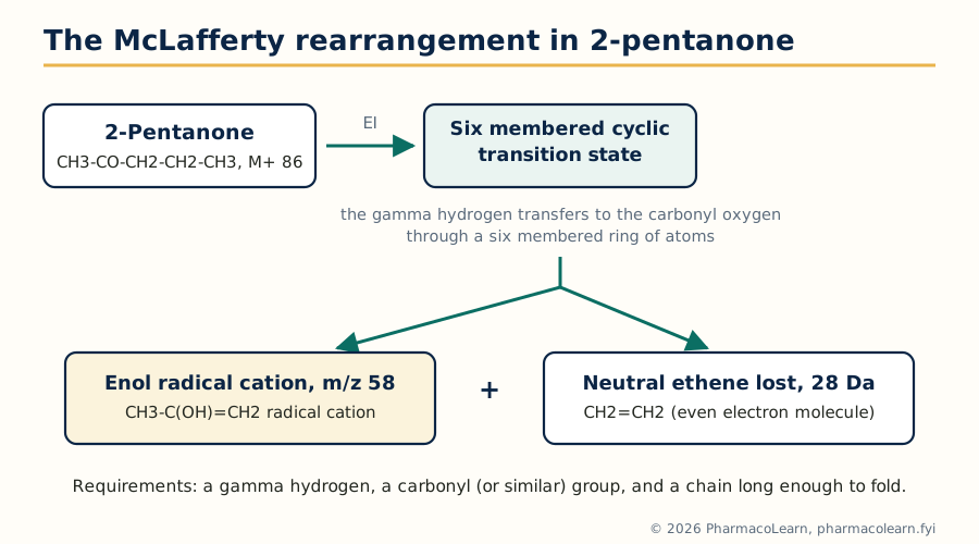 Figure: The McLafferty rearrangement. Six membered transition state, gamma hydrogen transfer, alpha-beta bond cleavage: the three features every answer must name.
Note the bookkeeping, because examiners probe it: the rearrangement ion is a radical cation (odd electron) formed from a radical cation by loss of an even electron neutral, which the even electron rule permits. A McLafferty peak therefore also proves a chain of at least three carbons beyond the carbonyl on one side, structural information from a single peak.
3.7 Metastable ions
Some ions survive the ion source but fall apart in the field free region between source and analyser. Their fragments appear not at the true fragment mass but as broad, low, diffuse peaks at an apparent mass m* given by:
m = (m2 squared) / m1*
where m1 is the decomposing parent and m2 the daughter. The classic example sits in the spectrum of toluene: the tropylium ion at 91 loses acetylene to give the cyclopentadienyl cation at 65, and the metastable peak appears at 65 x 65 / 91 = 46.4. A metastable peak is a certificate of parentage: it proves that a specific daughter came from a specific parent in one step, something intensities alone can never show. In interpretation, when two fragmentation routes to the same fragment compete, a metastable peak settles which one actually operates.
3.8 Isotopic peaks
The peaks one and two mass units above any ion are not noise; they are the isotope pattern, and they count atoms. Carbon-13 makes M+1 about 1.1 percent of M per carbon atom, so the M+1 height estimates the carbon count of the ion (and of the molecule, applied to M+). The M+2 peak carries the halogen signatures: chlorine (chlorine-35 and chlorine-37 in a 75.8 to 24.2 natural ratio) gives M : M+2 about 3 : 1 for one chlorine, and about 9 : 6 : 1 across M, M+2, M+4 for two; bromine (79 and 81 in a 50.7 to 49.3 ratio) gives M : M+2 about 1 : 1; two bromines give 1 : 2 : 1. Sulfur adds about 4.4 percent at M+2 per atom from sulfur-34, a quieter but useful signal.
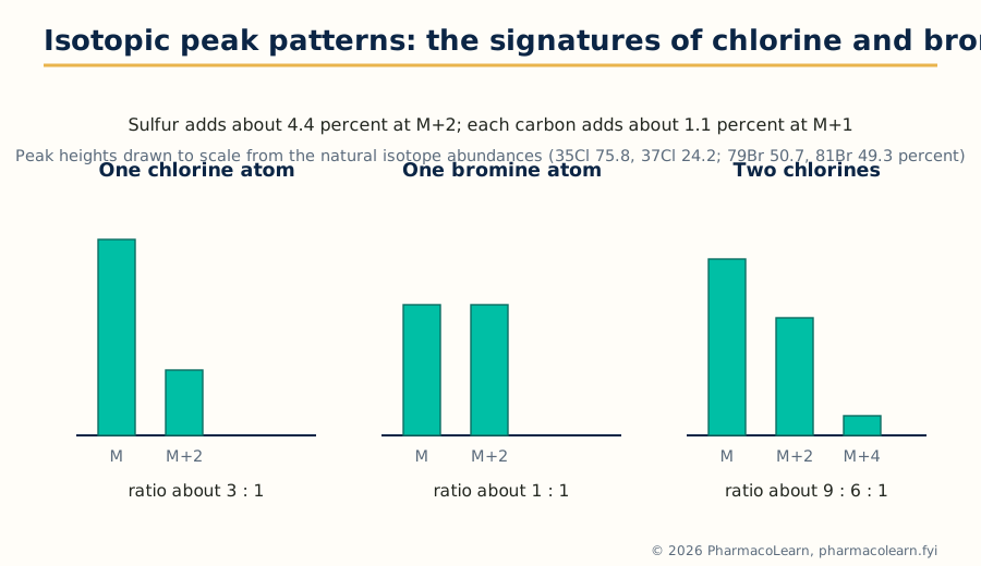 Figure: Isotope signatures. These patterns are visible in every fragment ion that retains the halogen, not only in the molecular ion.
The patterns apply to fragments as well as to M+, which multiplies their value: if the molecular ion shows one chlorine and a fragment at some lower mass still shows the 3 : 1 pair, that fragment retains the chlorine; if the pair vanishes below a certain fragment, the chlorine left with the neutral loss. Few single observations in mass spectrometry buy so much structural information so cheaply.
3.9 Interpretation workflow: a worked spectrum
1. Find M+: apply the nitrogen rule; read DBE from it
2. Read M+1 (carbon count) and M+2 (Cl, Br, S)
3. List the major fragments; note neutral losses
   (15 CH3, 18 H2O, 28 CO/C2H4, 29 CHO/C2H5, 31 OCH3,
    43 C3H7/CH3CO, 45 COOH/OC2H5 ...)
4. Match fragments to the alpha cleavage and McLafferty
   fingerprints of the groups IR has already suggested
5. Use metastables, where present, to certify key steps
6. Assemble a structure; check EVERY major peak is explained
   and the DBE and nitrogen rule are satisfied
Worked example: acetophenone. M+ at 120, strong; base peak 105; further peaks at 77 and 51; M+1 about 8.8 percent of M+. Nitrogen rule: even mass, zero or even nitrogens. M+1 suggests 8 carbons (8 x 1.1 = 8.8). A formula of C8H8O fits the mass (96 + 8 + 16 = 120) and gives DBE = 8 - 4 + 1 = 5. IR (given with the problem) shows a conjugated carbonyl near 1685 cm-1 and aromatic bands. Fragment 105 is M - 15, loss of a methyl radical: alpha cleavage of a methyl ketone, giving the benzoyl cation C6H5CO+, resonance stabilised and rightly the base peak. Fragment 77 is 105 - 28, loss of CO from the benzoyl ion, leaving the phenyl cation; 51 is 77 - 26, loss of acetylene from the phenyl cation, the standard aromatic cascade. The four DBE beyond the carbonyl are the benzene ring. Structure: C6H5COCH3, acetophenone, with every major peak assigned and every rule satisfied. That completeness, not the answer alone, is what full marks look like in this unit.
Unit 4: Hyphenated Chromatographic Techniques
4.1 Why hyphenate: separation meets identification
A chromatograph separates a mixture and reports peaks in time; a spectrometer identifies compounds but struggles with mixtures. A hyphenated technique welds the two together in line: the chromatograph delivers pure components one at a time, and the spectrometer identifies each as it emerges. Every system in this unit is that idea in a different costume, and every one of them turns on the same engineering problem, the interface: the junction that must transfer analyte from the separation conditions (a pressurised liquid, a gas stream, an electrophoresis buffer) into the detector's conditions without losing resolution or analyte. Judging each technique means asking three questions: what does the separation side do well, what does the detector side add, and what does the interface cost?
4.2 GC-MS
Gas chromatography separates volatile, thermally stable compounds on a capillary column in a helium or hydrogen stream; the mass spectrometer at the exit ionises each eluting component, usually by electron ionisation, and records a full mass spectrum per peak. The interface is the easiest in this unit because the GC effluent is already a dilute gas at low flow: a heated transfer line leads the column effluent straight into the ion source, sometimes through a jet separator that enriches analyte over carrier gas in older designs. The product of a run is a total ion chromatogram (peak per component) plus a searchable EI spectrum for each peak: library matching against collections of hundreds of thousands of reference spectra makes GC-MS the most confident routine identifier of volatile organics. Applications in pharmaceutical work: residual solvents, volatile impurities and degradation products, essential oil and flavour profiling, forensic and doping control samples, and environmental contaminants in raw materials. Its boundary is absolute: compounds that will not vaporise intact cannot be run, which is why the pharmaceutical mainstream lives in the next system instead.
4.3 LC-MS
Liquid chromatography handles the non-volatile, polar and fragile majority of drug molecules, and coupling it to MS was historically the hardest interface problem in analytical chemistry: about a millilitre per minute of liquid must become ions in a high vacuum. The solution is the atmospheric pressure interface. In electrospray ionisation (ESI) the eluent sprays through a charged needle, forming charged droplets that evaporate until gas phase ions, typically protonated molecules [M+H]+, are released at atmospheric pressure and sampled through a small orifice into the vacuum. In atmospheric pressure chemical ionisation (APCI) the eluent is vaporised in a heated nebuliser and ionised by a corona discharge, suiting smaller, less polar molecules. Because these are soft ionisation methods, spectra are simple, often a single molecular ion species, which makes LC-MS superb for molecular weight confirmation and quantification but poorer than EI for library style structural matching; tandem MS (MS/MS) restores structural information by fragmenting selected ions in a collision cell.
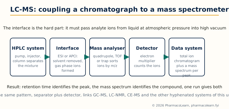 Figure: The LC-MS chain. The interface, not the analyser, is the invention that made the technique routine.
Pharmaceutical applications dominate modern analysis: impurity identification in drug substance and product, metabolite profiling in discovery and development, bioanalysis of drugs in plasma for pharmacokinetic studies (usually triple quadrupole MS/MS in selected reaction monitoring mode), peptide and protein characterisation, and cleaning validation. LC-MS is the default hyphenation against which the others in this unit are the specialists.
4.4 GC-AAS
Coupling gas chromatography to atomic absorption spectrometry answers a question neither instrument answers alone: not how much of an element a sample contains, but in which chemical forms. The GC separates volatile organometallic species; the effluent passes into a heated quartz furnace in the AAS light path, where the compounds are atomised and the element specific absorption is measured. The classic applications are speciation studies: methylmercury versus inorganic mercury in biological and environmental samples, alkyllead compounds, and organotin species. In pharmaceutical quality work its niche is elemental impurity speciation where the toxicology depends on the form, over and above the total element content that pharmacopoeial elemental impurity tests report. Sensitivity is high for the target element and the chromatogram contains only peaks of that element, a clean speciation fingerprint.
4.5 LC-FTIR
An infrared spectrum gives functional group proof that MS cannot, so LC-FTIR aims to record IR spectra of HPLC peaks. The obstacle is the solvent: water and the common mobile phases absorb IR radiation intensely and swamp the analyte. Two interface philosophies exist. Flow cell interfaces pass the eluent through a short path cell in the FTIR beam, workable only with IR transparent solvents and limited sensitivity. Solvent elimination interfaces deposit the eluent on a moving substrate (a rotating disc or a zinc selenide window), evaporate the solvent under vacuum and gentle heat, and measure the deposited analyte spots by reflectance or transmission, building a chromatogram from reconstructed IR responses (a Gram-Schmidt plot) with a full spectrum stored for every point. Solvent elimination wins on sensitivity and solvent freedom, including reversed phase gradients, and its applications are polymer additive analysis, drug-excipient compatibility studies and isomer discrimination, where IR distinguishes compounds whose mass spectra are nearly identical.
4.6 LC-NMR
NMR is the most informative and least sensitive of the spectroscopies, and LC-NMR exists to put that information onto HPLC peaks, typically for natural product isolation and metabolite identification, where an unknown's structure must be solved from micrograms. The interface is a flow probe: a small volume flow cell (typically 60 to 120 microlitres of active volume) sits in the magnet, connected to the column by narrow capillary tubing chosen to preserve chromatographic resolution. Operation modes trade time for spectrum quality: continuous flow for a first survey, stopped flow, in which the pump halts with the peak parked in the cell so long 1-D and even 2-D experiments can accumulate, and loop storage, in which peaks are parked in capillary loops for offline measurement. Two practical burdens define the technique: solvent signals must be suppressed (deuterated solvents are expensive at HPLC flow rates, so pulse sequence suppression of protonated solvent peaks is standard), and sensitivity demands concentrated peaks, often from repeated injections. Where it succeeds, the payoff is the complete Unit 2 argument, COSY, HSQC and HMBC included, performed on a component that was never isolated by hand.
4.7 CE-MS
Capillary electrophoresis separates by charge to size ratio in a narrow fused silica capillary under a high voltage, consuming nanolitres and giving exceptional plate counts for ionic species: peptides, oligonucleotides, charged metabolites and chiral separations with selector additives. Coupling to MS through an electrospray interface must respect the tiny CE flow (nanolitres per minute): a coaxial sheath liquid interface adds a make up flow around the capillary tip that both completes the electrical circuit and feeds the spray, at some cost in dilution; sheathless porous tip interfaces avoid the dilution for maximum sensitivity. Applications follow CE's strengths: charge variant profiling of therapeutic proteins, peptide mapping, metabolomics of ionic metabolites, and counter ion and small ion analysis. CE-MS is the specialist hyphenation for samples that are ionic, scarce and badly served by reversed phase LC.
4.8 HPTLC
High performance thin layer chromatography modernises the plate: finer, more uniform silica layers on glass or foil, instrumental sample application as narrow bands, controlled chamber development, and evaluation by scanning densitometry in absorbance or fluorescence. Identity is carried by the Rf value plus in situ spectra: the densitometer can record a UV spectrum of a spot on the plate, and plates can be eluted into a mass spectrometer through commercial elution interfaces for confirmation. Its pharmaceutical stronghold is herbal drug and Ayurvedic analysis, where pharmacopoeias prescribe HPTLC fingerprints for identity of crude drugs and extracts, alongside related substances testing and formulation assays where its virtues matter: many samples run side by side on one plate, minimal solvent use, the whole chromatogram permanently stored on the plate, and low cost per sample. As a screening and fingerprinting hyphenation (TLC with spectroscopic evaluation) it complements, rather than competes with, the column systems.
4.9 Supercritical fluid chromatography
SFC uses a supercritical fluid, in practice carbon dioxide above its critical point (31.1 degrees Celsius, 73.8 bar), as the main mobile phase component, usually with a polar modifier such as methanol and sometimes an additive. The fluid's low viscosity and high diffusivity give fast, high efficiency separations at several times HPLC speeds, and decompression returns the CO2 to a gas that simply leaves, simplifying fraction collection. Detection is by UV in routine work, with MS coupling straightforward because the decompressed stream suits atmospheric pressure ionisation. Its flagship pharmaceutical application is chiral separation: SFC on chiral stationary phases is the first choice for enantiomer analysis and preparative enantiomer purification in discovery chemistry, where its speed and easy solvent removal save days. It also serves lipophilic compound classes poorly retained in reversed phase, such as fat soluble vitamins, steroids and triglyceride type lipids.
4.10 Ion chromatography and ion exclusion chromatography
Ion chromatography is ion exchange chromatography engineered for sensitive ion measurement: low capacity exchangers, an eluent of dilute hydroxide or carbonate, and, in the standard suppressed mode, a suppressor device that converts the eluent to a low conductivity form (water or carbonic acid) while converting analyte ions to their more conducting acid or base forms, read by a conductivity detector. It quantifies anions (fluoride, chloride, nitrite, nitrate, phosphate, sulfate) and cations (sodium, potassium, ammonium, calcium, magnesium) at trace levels, serving water for pharmaceutical purposes testing, counter ion assay of drug salts, and ionic impurities. Ion exclusion chromatography separates by a different mechanism on a fully sulfonated cation exchanger: strong acids are excluded from the resin pores by Donnan exclusion and elute early, while weak acids partition into the pore liquid according to their ionisation and elute later, separated essentially by pKa. Its home ground is the profiling of weak organic acids, in fermentation broths, foods and pharmaceutical formulations, with conductivity or UV detection.
4.11 Flash chromatography
Flash chromatography is the preparative member of the list: column chromatography accelerated by moderate pressure (typically a few bar of air or nitrogen) pushing solvent through a cartridge of silica gel of defined particle size, following the method popularised by Still. Modern systems automate it: prepacked disposable cartridges, gradient pumps, UV (and often evaporative light scattering) detection, and fraction collection triggered by the detector trace. It is not an identification technique; its place in this unit is as the isolation engine that feeds every other technique. Reaction mixtures from medicinal chemistry are purified in minutes, natural product extracts are fractionated into testable components, and the purified outputs go forward to NMR and MS for the structural arguments of Units 2 and 3. Scale up is by cartridge size, from milligrams to hundreds of grams.
4.12 Choosing the hyphenated system
| Analytical problem | First choice | Why |
|---|---|---|
| Volatile, thermally stable unknowns | GC-MS | EI library spectra identify directly |
| Polar, fragile or high mass analytes; bioanalysis | LC-MS (ESI, MS/MS) | Soft ionisation, sensitivity, quantification |
| Elemental speciation (which form of the metal) | GC-AAS | Element specific detection after separation |
| Functional group proof for an LC peak; isomer cases | LC-FTIR | IR evidence MS cannot give |
| Full structure of an unisolated natural product | LC-NMR (stopped flow) | Complete NMR without manual isolation |
| Ionic metabolites, protein charge variants | CE-MS | Charge based separation, minute samples |
| Herbal identity fingerprints, many samples cheaply | HPTLC | Parallel samples, pharmacopoeial fingerprints |
| Enantiomers, fast purification of isomers | SFC | Chiral phases, speed, easy recovery |
| Trace anions and cations; drug salt counter ions | Ion chromatography | Suppressed conductivity sensitivity |
| Weak organic acid profiles | Ion exclusion chromatography | Separation by pKa |
| Purification before identification | Flash chromatography | Fast, automated, scalable isolation |
The pattern to carry into examinations: name the analyte class and the question first, and the technique follows. Hyphenation questions are almost never asking for instrument trivia; they are asking whether the candidate can match a separation mechanism and a detector to a stated problem.
Unit 5: Thermal Methods, Raman Spectroscopy and Immunoassay
5.1 Thermal analysis: the family and the thermogram
Thermal methods watch a sample while its temperature is driven through a programme, usually a steady heating ramp, and record some physical property against temperature. The record is a thermogram, and its steps, peaks and plateaus are the events of the sample's thermal life: melting, crystallisation, desolvation, decomposition, glass transition. Three techniques cover the syllabus: DSC measures heat flow, DTA measures a temperature difference, and TGA measures mass. Between them they answer the pharmaceutical questions of purity, polymorphism, solvate content, stability and compatibility that no spectrum addresses directly.
5.2 Differential scanning calorimetry
In DSC the instrument works to keep the sample and an inert reference following the same temperature programme, and records the heat flow needed to do so. Two designs achieve it. In heat flux DSC, sample and reference sit on a common thermoelectric disc inside one furnace, and the temperature difference between them, measured by thermocouples, is converted to heat flow. In power compensation DSC, separate small furnaces heat sample and reference, and the instrument varies their relative power to hold both at the same temperature; the power difference is the signal. On the thermogram, an endotherm (melting, desolvation) appears as a peak in one direction and an exotherm (crystallisation, decomposition, curing) as a peak in the other, by the plotting convention of the instrument.
The events read from a drug's DSC curve are standard: the melting endotherm, whose onset gives the melting point and whose area gives the enthalpy of fusion; the glass transition of an amorphous material, a step change in the baseline (a change in heat capacity, not a peak) at Tg; crystallisation exotherms when a metastable or amorphous form orders itself on heating; and separate endotherms for different polymorphs or for desolvation before melting. The flagship quantitative application is purity determination by the van't Hoff method: a small amount of impurity depresses and broadens the melting endotherm in a mathematically defined way, so the shape of a single melt yields a purity figure, the DSC purity assay used for reference standards. Pharmaceutical applications complete the list: polymorph screening and identification, drug-excipient compatibility screening (a shifted or vanished drug endotherm in a mixture warns of interaction), amorphous content estimation, and lyophilisation cycle design through the glass transition of the frozen concentrate.
5.3 Differential thermal analysis
DTA is the older and simpler instrument: sample and reference are heated in the same furnace with a thermocouple in each, and the recorded signal is simply the temperature difference (delta T) between them. When the sample melts, it lags behind the reference and an endothermic dip appears; when it crystallises or reacts exothermically, it runs ahead and a peak appears. DTA detects the same family of events as DSC, transitions, reactions and decompositions, and historically mapped the phase behaviour of minerals, clays and polymers. Its limitations against DSC are quantitative: delta T depends on sample packing, thermal conductivity and thermocouple placement, so enthalpies from DTA are approximate, and the baseline is less stable. The honest summary for an exam answer: DTA tells you at what temperature things happen, DSC tells you that and how much heat they involve; pharmaceutical laboratories therefore buy DSC, and DTA survives in high temperature materials work (its furnaces reach temperatures DSC designs do not) and as the conceptual parent of the family.
5.4 Thermogravimetric analysis
TGA records the mass of a sample continuously on a sensitive microbalance (the thermobalance) while the temperature programme runs, in a controlled atmosphere of nitrogen, air or oxygen chosen to suit the question. The thermogram is a descending staircase: each step is a mass loss event with an onset temperature and a percentage, and the derivative curve (DTG) resolves overlapping steps into peaks. Reading percentages against candidate stoichiometries is the interpretation skill: a first step of about 5 percent near 100 degrees in a hydrate whose formula weight predicts one water of crystallisation confirms the monohydrate; a plateau until 250 degrees followed by a single large step signals a stable anhydrous compound that decomposes without melting events interfering. Pharmaceutical applications: solvate and hydrate quantification (the standard check for how much solvent a crystal lattice holds), moisture and volatile content, decomposition kinetics and shelf life prediction from isothermal and ramped studies, ash and inorganic residue estimation, and oxidative stability comparisons between formulations. Coupling TGA to FTIR or MS of the evolved gases (an echo of Unit 4's hyphenation principle) identifies what each step actually loses.
5.5 Raman spectroscopy
Raman spectroscopy shines monochromatic light, in practice a laser, on the sample and analyses the tiny fraction of light scattered with a change of wavelength. Most scattering is Rayleigh scattering at the incident wavelength; about one photon in a million scatters inelastically. If the photon gives energy to a molecular vibration, the scattered light loses that energy and appears at longer wavelength: a Stokes line. If it collects energy from an already vibrating molecule, it gains energy: an anti-Stokes line, weaker because few molecules are vibrationally excited at room temperature. The Raman shift, the distance of these lines from the Rayleigh line in wavenumbers, equals the vibrational frequency, so the Raman spectrum, like the IR spectrum, is a vibrational fingerprint.
The instrumentation follows from the physics: a laser source (common choices include 532 and 785 nm diode or solid state lasers; 1064 nm excitation in FT-Raman instruments suppresses fluorescence), a filter or monochromator to reject the overwhelming Rayleigh line, and a sensitive CCD detector. The 785 nm laser is the pharmaceutical workhorse because it balances scattering strength against the fluorescence that ruins many 532 nm spectra of coloured drug samples. Applications play to Raman's peculiar strengths: water is a very weak Raman scatterer, so aqueous systems and biological samples are easy; no sample preparation is needed and measurements pass through glass vials and blister packs; and the technique distinguishes polymorphs crisply, which has made handheld Raman analysers standard for raw material identity verification in warehouse receiving, for counterfeit drug screening in the field, and for process monitoring (PAT) of blending and coating.
5.6 Raman versus IR: one vibrational truth, two selections
| Aspect | Infrared | Raman |
|---|---|---|
| Physical event | Absorption of IR radiation | Inelastic scattering of laser light |
| Selection rule | Vibration must change the dipole moment | Vibration must change the polarisability |
| Strong for | Polar bonds: O-H, N-H, C=O | Non-polar bonds: C=C, C-C, S-S, ring modes |
| Water as solvent | Very strong absorber, hostile | Very weak scatterer, friendly |
| Sample needs | Thin film, pellet, ATR contact | None; through glass is fine |
| Symmetric stretches | Often weak or inactive | Often strong |
| Main practical enemy | Water and CO2 bands | Sample fluorescence |
The two spectra are complementary in the strict sense: for a molecule with a centre of symmetry, vibrations are active in one technique or the other, never both (the mutual exclusion rule), and in ordinary molecules the strong IR bands and strong Raman bands still tend to be different vibrations. An identification argued from both spectra is correspondingly harder to shake, which is why pharmacopoeial identification strategies increasingly pair them.
5.7 Biological standardization and bioassay
Some drug activities, historically those of complex natural products and biologicals, could not be measured by any chemical or physical test: the only assay was the biological response itself. Biological standardization therefore compares the preparation against a stable reference standard of the same substance in a defined biological system and expresses potency in units relative to that standard. A bioassay is designed as a comparative experiment: graded doses of standard and test are given to groups of animals, cells or tissues; responses are measured; and the potency ratio is computed from the parallel dose response lines, with statistical checks for parallelism and linearity that validate the assay. Designs include quantal (all or none response, such as death or protection) and graded (measured response, such as blood pressure change or blood sugar fall) endpoints, and the classical matched bracket and Latin square layouts that cancel biological variation. The insulin assay by blood sugar lowering in rabbits and the digitalis assay by cardiac effect were the pharmacopoeial mainstays of this approach, and they form the bridge to the immunoassay methods that largely replaced them.
5.8 ELISA
Enzyme linked immunosorbent assay replaces the animal and the radioactive label with an enzyme label and a coloured product. The architecture is general: an antibody (or antigen) is immobilised on the wells of a microplate; the sample's analyte binds; an enzyme conjugated second reagent completes the chosen format; washing separates bound from free; and the enzyme's substrate is converted to a coloured (or fluorescent, or luminescent) product read in a plate reader. Formats matter and should be named correctly. In a sandwich ELISA the analyte is caught between an immobilised capture antibody and an enzyme labelled detection antibody, giving high specificity for larger analytes with two epitopes. In a competitive ELISA sample analyte competes with a labelled or immobilised reference, so the signal falls as analyte rises, the format used for small molecules with a single epitope. Pharmaceutical and clinical uses surround the student: cytokine and biomarker measurement, anti-drug antibody testing for biologics, residual host cell protein assays in biomanufacturing, vaccine potency support, and screening of hybridomas in antibody production.
5.9 Radioimmunoassay: principle, and the assays of insulin and digitalis
Radioimmunoassay (RIA), developed by Yalow and Berson for plasma insulin, measures minute concentrations by competition. A fixed, limited amount of specific antibody is incubated with a fixed amount of radioactively labelled antigen (classically iodine-125 labelled) and the sample, whose unlabelled antigen competes for the same binding sites. The more analyte in the sample, the less label is bound. Bound and free fractions are separated, the radioactivity of one fraction is counted, and the result is read from a calibration curve; signal therefore falls as concentration rises, the inverse calibration that defines all competitive assays.
The insulin assay was the founding application: plasma insulin at picomolar levels, far below chemical detection, became measurable, transforming diabetes research. The digitalis (digoxin) assay is the clinical exemplar: digoxin's therapeutic window is narrow and its toxicity dangerous and mimics the disease treated, so serum digoxin monitoring by RIA (and its successors) became routine, with the assay's cross reactivity toward digoxin metabolites and endogenous digoxin like immunoreactive substances taught as its known weakness. RIA's costs are the ones that displaced it: radioisotope handling and licensing, short reagent shelf life set by isotope decay, and waste disposal. Its sensitivity and specificity survive in the ELISA and chemiluminescent assays that inherited its competitive and sandwich logic, and the syllabus retains it because the principle, limited antibody plus competing labelled ligand, remains the template for all binding assays.
5.10 Choosing among the Unit 5 methods
QUESTION                                        METHOD
At what temperature does it melt, change     DSC (events and
form or lose its solvent, and with           enthalpies),
how much heat?                               DTA (events only)
How much hydrate, solvent or volatile        TGA (mass steps
matter, and at what temperature lost?        read as percentages)
Is this raw material the right polymorph,    Raman (through the
checked through its container?               container, no prep)
Is the hormone, drug or antibody present     Immunoassay:
at trace level in a biological fluid?        RIA historically,
                                             ELISA in modern form
Taken as a whole, Unit 5 teaches a habit rather than a hierarchy: match the physical observable (heat, mass, scattered light, binding) to the property the question actually asks about, exactly as Unit 4 matched separations to detectors.
Frequently Asked Questions
Q: How do the Woodward-Fieser rules distinguish a homoannular from a heteroannular diene, and why does it matter numerically?
A homoannular diene has both double bonds in the same ring and starts from a base value of 253 nm; a heteroannular diene has them in different rings (or is acyclic) and starts from 214 nm. The 39 nm difference is the largest single decision in the calculation, so misclassifying the diene wrecks the prediction before any increment is added. The higher homoannular value reflects its fixed cisoid geometry, which holds the pi systems coplanar and conjugating at maximum effectiveness.
Q: A calculated lambda max comes out 20 nm away from the observed band. What are the likely causes?
Four usual suspects, in order: the diene or enone class was misread (homoannular versus heteroannular, five versus six membered enone ring); a substituent was miscounted, typically ring residues at a ring junction carbon or an exocyclic double bond that counts for two rings; the solvent correction was omitted or applied with the wrong sign; or the real chromophore is twisted out of planarity by steric crowding, which genuinely breaks the rules' assumption of coplanar conjugation. A 20 nm miss is diagnostic information, not arithmetic failure.
Q: Why has ATR largely replaced the KBr pellet in routine IR work?
ATR needs no preparation: the sample is pressed against the crystal and measured as it is, including pastes, films, liquids and aqueous samples that a pellet cannot handle, because the evanescent wave samples only about a micrometre of depth and water never gets a long path to absorb through. The pellet's grinding, drying and pressing steps, and its moisture artefacts, disappear. The honest trade offs are that ATR sees the surface rather than the bulk, and its relative band intensities differ slightly from transmission spectra, so reference matching should use ATR libraries.
Q: COSY, HSQC and HMBC are all run on one unknown. What does each one prove that the others cannot?
COSY proves which protons are coupled, tracing runs of neighbouring CH groups, but it stops dead at heteroatoms and quaternary carbons. HSQC proves which proton sits on which carbon, assigning every protonated carbon, but says nothing about how the groups connect. HMBC proves the connections across the gaps: its two and three bond correlations leap heteroatoms and quaternary centres and place carbonyls and ring junctions. A structure is solved when the COSY chains, the HSQC assignments and the HMBC bridges are all consistent with one skeleton.
Q: Why is INADEQUATE so rarely run if it gives the carbon skeleton directly?
Sensitivity. The experiment needs two carbon-13 nuclei bonded to each other; at 1.1 percent natural abundance only about one molecule in ten thousand qualifies for any given bond, so the signals are extremely weak and demand concentrated samples and many hours of acquisition. It is kept for structures that defeat indirect methods, novel natural products and disputed skeletons, where one overnight spectrum settles what weeks of inference could not.
Q: How do you tell an alcohol from an amine by mass spectrometry alone?
Both fragment by alpha cleavage, but the charge bearing fragments differ by one mass unit: a primary alcohol gives the oxonium ion CH2=OH+ at m/z 31, while a primary amine gives the iminium ion CH2=NH2+ at m/z 30, usually its base peak. The molecular ion adds the second test: an amine with one nitrogen has an odd molecular weight by the nitrogen rule, an alcohol's is even. Together, base peak 30 versus 31 and odd versus even M+, the distinction is unambiguous.
Q: What does a metastable peak prove, and how is its position calculated?
It proves parentage: that a particular daughter ion was formed from a particular parent ion in a single step in the field free region, rather than in the source among many possible routes. Its apparent mass is m* = (m2 squared)/m1, daughter mass squared divided by parent mass. The textbook example is toluene: tropylium 91 decomposing to 65 gives a broad metastable peak at 46.4, certifying the loss of acetylene from the tropylium ion.
Q: An unknown's mass spectrum shows M and M+2 in a ratio of about 9 to 6 to 1 including an M+4 peak. What is in the molecule?
Two chlorine atoms. One chlorine gives 3 : 1 across M and M+2 only; two chlorines multiply the pattern out to M+4 with intensities following the binomial expansion of the 3 : 1 ratio, giving approximately 9 : 6 : 1. One bromine would give 1 : 1, and two bromines 1 : 2 : 1, so the M+4 peak with that intensity profile is a chlorine pair's signature. The same pattern check on fragment ions shows which fragments retain both chlorines.
Q: Why is LC-MS, and not GC-MS, the default hyphenated technique in pharmaceutical analysis?
Because most drug molecules and their impurities are polar, thermally fragile or insufficiently volatile, and GC demands that an analyte vaporise intact. LC separates exactly the compounds GC cannot touch, and electrospray ionisation hands them to the mass spectrometer as intact protonated molecules, with MS/MS available for structure and for sensitive bioanalysis. GC-MS remains superior for volatile compounds, where its EI libraries identify peaks outright, but that is the minority of pharmaceutical work.
Q: DSC and DTA both heat a sample beside a reference. What does DSC measure that DTA does not, and why did DSC win in pharmaceutical laboratories?
DTA records only the temperature difference between sample and reference, which marks the temperatures of events but gives unreliable enthalpies because the signal depends on packing and thermal contact. DSC, whether heat flux or power compensation design, measures heat flow quantitatively, so the same run returns transition temperatures and the enthalpies behind them, enabling melting point and enthalpy of fusion from one curve and purity by the van't Hoff treatment of the melt shape. Pharmaceutical questions are quantitative (how pure, how much amorphous, how much hydrate with TGA alongside), so DSC displaced DTA except in high temperature materials work.
Complete MPC201T notes, all 5 units in one PDF, free to keep.
Other M.Pharm subjects: MPH101T · MPC101T · MPL101T · MPH102T · MPH103T · MPH104T · MPL102T · MPL103T · MPL104T · MPC102T · MPC103T · MPC104T · MPH201T · MPH202T · MPH203T · MPH204T · MPC201T · MPC202T · MPC203T · MPC204T · M.Pharm